5. Run-time analysis

5.1. General remarks

Frequently, the numerical treatment of scientific problems can lead to time-consuming code and the question arises how its performance can be improved. There exist a variety of different kinds of approaches. One could for example choose to make use of more powerful hardware or distribute the task on numerous compute nodes of a compute cluster. Even though today, human resources tend to be more costly than hardware resource, the latter should not be wasted by very inefficient code.

In certain cases, speed can be improved by making use of graphical processors (GPU) which are able to handle larger data sets in parallel. While writing code for GPUs may be cumbersome, there exists for example the CuPy library [1] which can serve as a drop-in replacement for most of the NumPy library and will run on NVIDIA GPUs.

On the software side, an option is to make use of optimized code provided by numerical libraries like NumPy and SciPy discussed in Section 4. Sometimes, it can make sense to implement particularly time-consuming parts in the programming language C for which highly optimizing compilers are available. This approach does not necessarily require to write proper C code. One can make use of Cython [2] instead, which will autogenerate C code from Python-like code.

Another option is the use of just in time (JIT) compilers as is done in PyPy [3] and Numba [4]. The latter is readily available through the Anaconda distribution and offers an easy approach to speeding up time-critical parts of the code by simply adding a decorator to a function. Generally, JIT compilers analyze the code before its first execution and create machine code allowing to run the code faster in subsequent calls.

While some of the methods just mentioned can easily be implemented, others may require a significant investment of time. One therefore needs to assess whether the gain in compute time really exceeds the cost in developer time. It is worth following the advice of the eminent computer scientist Donald E. Knuth [5] who wrote already 45 years ago [6]

There is no doubt that the grail of efficiency leads to abuse. Programmers waste enormous amounts of time thinking about, or worrying about, the speed of noncritical parts of their programs, and these attempts at efficiency actually have a strong negative impact when debugging and maintenance are considered. We should forget about small efficiencies, say about 97 % of the time: premature optimization is the root of all evil.

Yet we should not pass up our opportunities in that critical 3 %. A good programmer will not be lulled into complacency by such reasoning, he will be wise to look carefully at the critical code; but only after that code has been identified.

Before beginning to optimize code, it is important to identify the parts where most of the time is spent and the rest of this chapter will be devoted to techniques allowing to do so. At this point, it is worth emphasizing that a piece of code executed relatively fast can be more relevant than a piece of code executed slowly if the first one is executed very often while the second one is executed only once.

Code optimization often entails a risk for bugs to enter the code. Obviously, fast-running code is not worth anything if it does not produce correct results. It can then be very reassuring if one can rely on a comprehensive test suite (Section 3) and if one has made use of a version control system (Section 2) during code development and code optimization.

Before discussing techniques for timing code execution, we will discuss a few potential pitfalls.

5.2. Some pitfalls in run-time analysis

A simple approach to performing a run-time analysis of code could consist in taking the time before and after the code is executed. The time module in the Python standard library offers the possibility to determine the current time:

>>> import time
>>> time.ctime()
'Thu Dec 27 11:13:33 2018'

While this result is nicely readable, it is not well suited to calculate time differences. For this purpose, the seconds passed since the beginning of the epoch are better suited. On Unix systems, the epoch starts on January, 1970 at 00:00:00 UTC:

>>> time.time()
1545905769.0189064

Now, it is straightforward to determine the time elapsed during the execution of a piece of code. The following code repeats the execution several times to convey an idea of the fluctuations to be expected.

import time

for _ in range(10):
    sum_of_ints = 0
    start = time.time()
    for n in range(1000000):
        sum_of_ints = sum_of_ints + 1
    end = time.time()
    print(f'{end-start:5.3f}s', end='  ')

Executing this code yields:

0.142s  0.100s  0.093s  0.093s  0.093s  0.093s  0.092s  0.091s  0.091s  0.091s

Doing a second run on the same hardware, we obtained:

0.131s  0.095s  0.085s  0.085s  0.088s  0.085s  0.084s  0.085s  0.085s  0.085s

While these numbers give an idea of the execution time, they should not be taken too literally. In particular, it makes sense to average over several loops. This is facilitated by the timeit module in the Python standard library which we will discuss in the following section.

When performing run-time analysis as just described, one should be aware that a computer may be occupied by other tasks as well. In general, the total elapsed time will thus differ from the time actually needed to execute a specific piece of code. The time module therefore provides two functions. In addition to the time function which records the wall clock time, there exist a process_time function which counts the time attributed to the specific process running our Python script. The following example demonstrates the difference by intentionally letting the program pause for a second once in a while. Note, that although the execution of time.sleep occurs within the process under consideration, the time needed is ignored by process_time. Therefore, we can use time.sleep to simulate other activities of the computer, even if it is done in a somewhat inappropriate way.

import time

sum_of_ints = 0
start = time.time()
start_proc = time.process_time()
for n in range(10):
    for m in range(100000):
        sum_of_ints = sum_of_ints + 1
    time.sleep(1)
end = time.time()
end_proc = time.process_time()
print(f'total time:   {end-start:5.3f}s')
print(f'process time: {end_proc-start_proc:5.3f}s')

In a run on the same hardware as used before, we find the following result:

total time:   10.207s
process time: 0.197s

The difference basically consists of the ten seconds spent while the code was sleeping.

One should also be aware that enclosing the code in question in a function will lead to an additional contribution to the execution time. This particularly poses a problem if the execution of the code itself requires only little time. We compare the two scripts

import time

sum_of_ints = 0
start_proc = time.process_time()
for n in range(10000000):
    sum_of_ints = sum_of_ints + 1
end_proc = time.process_time()
print(f'process time: {end_proc-start_proc:5.3f}s')

and

import time

def increment_by_one(x):
    return x+1

sum_of_ints = 0
start_proc = time.process_time()
for n in range(10000000):
    increment_by_one(sum_of_ints)
end_proc = time.process_time()
print(f'process time: {end_proc-start_proc:5.3f}s')

Tht first script takes on average over 10 runs 0.9 seconds while the second script takes 1.1 seconds and thus runs about 20% slower.

Independently of the methods used and even if one of the methods discussed later is employed, a run-time analysis will always influence the execution of the code. The measured run time therefore will be larger than without doing any timing. However, we should still be able to identify the parts of the code which take most of the time.

A disadvantage of the methods discussed so far consists in the fact that they require a modification of the code. Usually, it is desirable to avoid such modifications as much as possible. In the following sections, we will present a few timing techniques which can be used according to the specific needs.

5.3. The timeit module

Short isolated pieces of code can conveniently be analyzed by functions provided by the timeit module. By default, the average code execution time will be determined on the basis of one million of runs. As a first example, let us determine the execution time for the evaluation of the square of 0.5:

>>> import timeit
>>> timeit.timeit('0.5**2')
0.02171438499863143

The result is given in seconds. In view of one million of code executions, we obtain an execution time of 22 nanoseconds. If we want to use an argument, we cannot define it in the outer scope:

>>> x = 0.5
>>> timeit.timeit('x**2')
Traceback (most recent call last):
  File "<stdin>", line 1, in <module>
  File "/opt/anaconda3/lib/python3.6/timeit.py", line 233, in timeit
    return Timer(stmt, setup, timer, globals).timeit(number)
  File "/opt/anaconda3/lib/python3.6/timeit.py", line 178, in timeit
    timing = self.inner(it, self.timer)
  File "<timeit-src>", line 6, in inner
NameError: name 'x' is not defined

Instead, we can pass the global namespace through the globals argument:

>>> x = 0.5
>>> timeit.timeit('x**2', globals=globals())
0.103586286000791

As an alternative, one can explicitly assign the variable x in the second argument intended for setup code. Its execution time is not taken into account:

>>> timeit.timeit('x**2', 'x=0.5')
0.08539198899961775

If we want to compare with the pow function of the math module, we have to add the import statement to the setup code as well:

>>> timeit.timeit('math.pow(x, 2)', 'import math; x=0.5')
0.2346674630025518

A more complex example of the use of the timeit module compares the evaluation of a trigonometric function by means of a NumPy universal function with the use of the corresponding function of the math module:

import math
import timeit
import numpy as np
import matplotlib.pyplot as plt

def f_numpy(nmax):
    x = np.linspace(0, np.pi, nmax)
    result = np.sin(x)

def f_math(nmax):
    dx = math.pi/(nmax-1)
    result = [math.sin(n*dx) for n in range(nmax)]

x = []
y = []
for n in np.logspace(0.31, 6, 300):
    nint = int(n)
    t_numpy = timeit.timeit('f_numpy(nint)', number=10, globals=globals())
    t_math = timeit.timeit("f_math(nint)", number=10, globals=globals())
    x.append(nint)
    y.append(t_math/t_numpy)

plt.rc('text', usetex=True)
plt.plot(x, y, 'o')
plt.xscale('log')
plt.xlabel('vector size', fontsize=20)
plt.ylabel(r'$t_\mathrm{math}/t_\mathrm{numpy}$', fontsize=20)
plt.show()

The result is displayed in Figure 5.1.

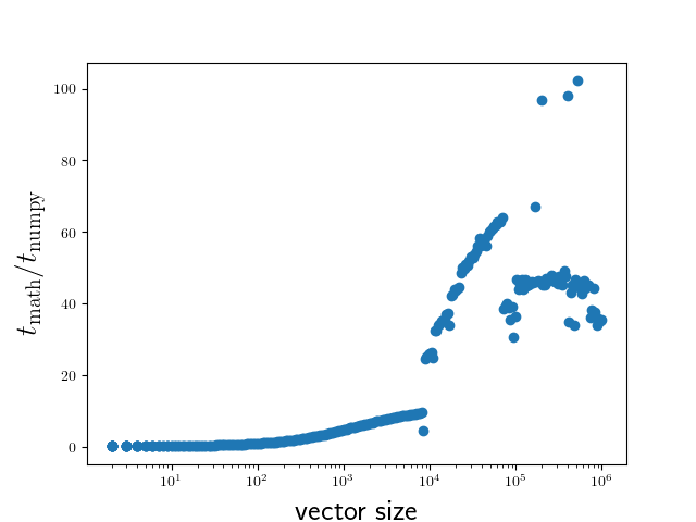
Figure 5.1 Comparison of execution times of the sine functions taken from the NumPy package and from the math module for a range of vector sizes.

We close this section with two remarks. If one wants to assess the fluctuations of the measure execution times, one can replace the timeit function by the repeat function:

>>> x = 0.5
>>> timeit.repeat('x**2', repeat=10, globals=globals())
[0.1035151930009306, 0.07390781700087246, 0.06162133299949346,
 0.05376200799946673, 0.05260805999932927, 0.05276966699966579,
 0.05227632500100299, 0.052304120999906445, 0.0523306600007345,
 0.05286436900132685]

For users of the IPython shell or the Jupyter notebook, the magics %timeit and %%timeit provide a simple way to time the execution of a single line of code or a code cell, respectively. These magics choose a reasonable number of repetitions to obtain good statistics within a reasonable amount of time.

5.4. The cProfile module

The timeit module discussed in the previous section is useful to determine the execution time of one-liners or very short code segments. It is not very useful though to determine the compute-time intensive parts of a bigger program. If the program is nicely modularized in functions and methods, the cProfile module will be of help. It determines, how much time is spent in the individual functions and methods and thereby gives valuable information about which parts will benefit from code optimization.

We consider as a specific example the quantum mechanical time evolution of a narrow Gaussian wave packet initially localized at the center of an infinite potential well [7]. The initial state is decomposed in the appropriately truncated eigenbasis of the potential well. Once the coefficients of the expansion are known, it is straightforward to determine the state at any later time. The time evolution of the probability density is shown in Figure 5.2.

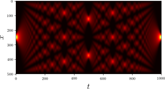
Figure 5.2 Time evolution of the probability density of an initial Gaussian wave packet positioned at the center of an infinite potential well. Brighter colors imply larger probability densities.

This figure has been obtained by means of the following Python script called carpet.py.

from math import cos, exp, pi, sin, sqrt
from cmath import exp as cexp
import numpy as np
import matplotlib.pyplot as plt
from matplotlib import cm

class InfiniteWell:
    def __init__(self, psi0, width, nbase, nint):
        self.width = width
        self.nbase = nbase
        self.nint = nint
        self.coeffs = self.get_coeffs(psi0)

    def eigenfunction(self, n, x):
        if n % 2:
            return sqrt(2/self.width)*sin((n+1)*pi*x/self.width)
        return sqrt(2/self.width)*cos((n+1)*pi*x/self.width)

    def get_coeffs(self, psi):
        coeffs = []
        for n in range(self.nbase):
            f = lambda x: psi(x)*self.eigenfunction(n, x)
            c = trapezoidal(f, -0.5*self.width, 0.5*self.width, self.nint)
            coeffs.append(c)
        return coeffs

    def psi(self, x, t):
        psit = 0
        for n, c in enumerate(self.coeffs):
            psit = psit + c*cexp(-1j*(n+1)**2*t)*self.eigenfunction(n, x)
        return psit

def trapezoidal(func, a, b, nint):
    delta = (b-a)/nint
    integral = 0.5*(func(a)+func(b))
    for k in range(1, nint):
        integral = integral+func(a+k*delta)
    return delta*integral

def psi0(x):
    sigma = 0.005
    return exp(-x**2/(2*sigma))/(pi*sigma)**0.25

w = InfiniteWell(psi0=psi0, width=2, nbase=100, nint=1000)
x = np.linspace(-0.5*w.width, 0.5*w.width, 500)
ntmax = 1000
z = np.zeros((500, ntmax))
for n in range(ntmax):
    t = 0.25*pi*n/(ntmax-1)
    y = np.array([abs(w.psi(x, t))**2 for x in x])
    z[:, n] = y
z = z/np.max(z)
plt.rc('text', usetex=True)
plt.imshow(z, cmap=cm.hot)
plt.xlabel('$t$', fontsize=20)
plt.ylabel('$x$', fontsize=20)
plt.show()

This code is by no means optimal. After all, we want to discuss strategies to find out where most of the compute time is spent and what we can do to improve the situation. Before doing so, let us get a general idea of how the code works.

The initial wave function is the Gaussian defined in the function psi0 in lines 40-42. Everything related to the basis functions is collected in the class InfiniteWell. During the instantiation, we define the initial wave function psi0, the total width of the well width, the number of basis states nbase, and the number of integration points nint to be used when determining the coefficients. The expansion coefficients of the initial state are determined in get_coeffs defined in lines 19-25 and called from line 12. The value of the eigenfunction corresponding to eigenvalue n at position x is obtained by means of the method eigenfunction defined in line 14-17. The integration is carried out very simply according to the trapezoidal rule as defined in function trapezoidal in lines 33-38. The wave function at a given point x and a given time t is calculated by method psi defined in lines 27-31. The code from line 44 to the end serves to calculate the time evolution and to render the image shown in Figure 5.2.

In this version of the code, we deliberately do not make use of NumPy except to obtain the image. Of course, NumPy would provide a significant speedup right away and one would probably never write the code in the way shown here. But it provides a good starting point to learn about run-time analysis. Where does the code spend most of its time?

To address this question, we make use of the cProfile module contained in the Python standard library. Among the various ways of using this module, we choose one which avoids having to change our script:

% python -m cProfile -o carpet.prof carpet.py

This command runs the script carpet.py under the control of the cProfile module. The option -o carpet.prof indicates that the results of this profiling run are stored in the file carpet.prof. This binary file allows to analyze the obtained data in various ways by means of the pstats module. Let us try it out:

  >>> import pstats
  >>> p = pstats.Stats('carpet.prof')
  >>> p.sort_stats('time').print_stats(15)
  Tue Jan 22 17:04:46 2019    carpet.prof

        202073424 function calls (202065686 primitive calls) in 633.175 seconds

  Ordered by: internal time
  List reduced from 3684 to 15 due to restriction <15>

  ncalls  tottime  percall  cumtime  percall filename:lineno(function)
50100100  232.867    0.000  354.468    0.000 carpet.py:14(eigenfunction)
  500000  184.931    0.000  623.191    0.001 carpet.py:27(psi)
50000000   84.417    0.000   84.417    0.000 {built-in method cmath.exp}
50100101   55.301    0.000   55.301    0.000 {built-in method math.sqrt}
25050064   33.170    0.000   33.170    0.000 {built-in method math.cos}
25050064   33.129    0.000   33.129    0.000 {built-in method math.sin}
       1    3.326    3.326    4.341    4.341 {built-in method exec_}
    1000    1.878    0.002  625.763    0.626 carpet.py:50(<listcomp>)
  503528    0.699    0.000    0.699    0.000 {built-in method builtins.abs}
    1430    0.372    0.000    0.372    0.000 {method 'read' of '_io.BufferedReader' objects}
  100100    0.348    0.000    1.386    0.000 carpet.py:22(<lambda>)
       2    0.300    0.150    0.300    0.150 {built-in method statusBar}
  100100    0.294    0.000    0.413    0.000 carpet.py:40(psi0)
     100    0.154    0.002    1.540    0.015 carpet.py:33(trapezoidal)
  100101    0.119    0.000    0.119    0.000 {built-in method math.exp}

After having imported the pstats module, we load our profiling file carpet.prof to obtain a statistics object p. The data can then be sorted with the sort_stats method according to different criteria. Here, we have chosen the time spent in a function. Since the list is potentially very long, we have restricted the output to 15 entries by means of the print_stats method.

Let us take a look at the information provided by the run-time statistics. Each line corresponds to one of the 15 most time-consuming functions and methods out of a total of 3695. The total time of about 667 seconds is mostly spent in the function psi listed in the second line. There are actually two times given here. The total time (tottime) of 196 seconds counts only the time actually spent inside the function. The time required to execute functions called from psi are not counted. In contrast, these times count towards the cumulative time (cumtime). An important part of the difference can be explained by the evaluation of the eigenfunctions as listed in the first line.

Since we have sorted according to time, which actually corresponds to tottime, the first line lists the method consuming most of the time. Even though the time needed per call is so small that it is given as 0.000 seconds, this function is called very often. In the column ncalls the corresponding value is listed as 50100100. In such a situation, it makes sense to check whether this number can be understood.

In a first step, the expansion coefficients need to be determined. We use 100 basis functions as specified by nbase and 1001 nodes which is one more than the value of nint. This results in a total of 100100 evaluations of eigenfunctions, actually less than a percent of the total number of evaluations of eigenfunctions. In order to determine the data displayed in Figure 5.2, we evaluate 100 eigenfunctions on a grid of size 500×1000, resulting in a total of 50000000 evaluations.

These considerations show that we do not need to bother with improving the code determining the expansion coefficients. However, the situation might be quite different if we would not want to calculate data for a relatively large grid. Thinking a bit more about it, we realize that the number of 50000000 evaluations for the time evolution is much too big. After all, we are evaluating the eigenfunctions at 500 different positions and we are considering 100 eigenfunctions, resulting in only 50000 evaluations. For each of the 1000 time values, we are unnecessarily recalculating eigenfunctions for the same arguments. Avoiding this waste of compute time could speed up our script significantly.

There are basically two ways to do so. We could restructure our program in such a way that we evaluate the grid for constant position along the time direction. Then, we just need to keep the values of the 100 eigenfunctions at a given position. If we want to have the freedom to evaluate the wave function at a given position and time on a certain grid, we could also store the values of all eigenfunctions at all positions on the grid in a cache for later reuse. This is an example of trading compute time against memory. We will implement the latter idea in the next version of our script listed below. [8]

from math import cos, exp, pi, sin, sqrt
from cmath import exp as cexp
import numpy as np
import matplotlib.pyplot as plt
from matplotlib import cm

class InfiniteWell:
    def __init__(self, psi0, width, nbase, nint):
        self.width = width
        self.nbase = nbase
        self.nint = nint
        self.coeffs = self.get_coeffs(psi0)
        self.eigenfunction_cache = {}

    def eigenfunction(self, n, x):
        if n % 2:
            return sqrt(2/self.width)*sin((n+1)*pi*x/self.width)
        return sqrt(2/self.width)*cos((n+1)*pi*x/self.width)

    def get_coeffs(self, psi):
        coeffs = []
        for n in range(self.nbase):
            f = lambda x: psi(x)*self.eigenfunction(n, x)
            c = trapezoidal(f, -0.5*self.width, 0.5*self.width, self.nint)
            coeffs.append(c)
        return coeffs

    def psi(self, x, t):
        if not x in self.eigenfunction_cache:
            self.eigenfunction_cache[x] = [self.eigenfunction(n, x)
                                           for n in range(self.nbase)]
        psit = 0
        for n, (c, ef) in enumerate(zip(self.coeffs, self.eigenfunction_cache[x])):
            psit = psit + c*ef*cexp(-1j*(n+1)**2*t)
        return psit

def trapezoidal(func, a, b, nint):
    delta = (b-a)/nint
    integral = 0.5*(func(a)+func(b))
    for k in range(1, nint):
        integral = integral+func(a+k*delta)
    return delta*integral

def psi0(x):
    sigma = 0.005
    return exp(-x**2/(2*sigma))/(pi*sigma)**0.25

w = InfiniteWell(psi0=psi0, width=2, nbase=100, nint=1000)
x = np.linspace(-0.5*w.width, 0.5*w.width, 500)
ntmax = 1000
z = np.zeros((500, ntmax))
for n in range(ntmax):
    t = 0.25*pi*n/(ntmax-1)
    y = np.array([abs(w.psi(x, t))**2 for x in x])
    z[:, n] = y
z = z/np.max(z)
plt.rc('text', usetex=True)
plt.imshow(z, cmap=cm.hot)
plt.xlabel('$t$', fontsize=20)
plt.ylabel('$x$', fontsize=20)
plt.show()

Now, we check in method psi whether the eigenfunction cache already contains data for a given position x. If this is not the case, the required values are calculated and the cache is updated.

As a result of this modification of the code, the profiling data change considerably:

Tue Jan 22 17:10:33 2019    carpet.prof

         52205250 function calls (52197669 primitive calls) in 185.581 seconds

   Ordered by: internal time
   List reduced from 3670 to 15 due to restriction <15>

   ncalls  tottime  percall  cumtime  percall filename:lineno(function)
   500000   97.612    0.000  177.453    0.000 carpet.py:28(psi)
 50000000   79.415    0.000   79.415    0.000 {built-in method cmath.exp}
     1000    2.162    0.002  180.342    0.180 carpet.py:54(<listcomp>)
        1    1.176    1.176    2.028    2.028 {built-in method exec_}
   503528    0.732    0.000    0.732    0.000 {built-in method builtins.abs}
   150100    0.596    0.000    0.954    0.000 carpet.py:15(eigenfunction)
   100100    0.353    0.000    1.349    0.000 carpet.py:23(<lambda>)
     1430    0.323    0.000    0.323    0.000 {method 'read' of '_io.BufferedReader' objects}
        2    0.301    0.151    0.301    0.151 {built-in method statusBar}
   100100    0.278    0.000    0.396    0.000 carpet.py:44(psi0)
   150101    0.171    0.000    0.171    0.000 {built-in method math.sqrt}
      100    0.140    0.001    1.489    0.015 carpet.py:37(trapezoidal)
   100101    0.119    0.000    0.119    0.000 {built-in method math.exp}
    75064    0.095    0.000    0.095    0.000 {built-in method math.sin}
    75064    0.093    0.000    0.093    0.000 {built-in method math.cos}

We observe a speed-up of a factor of 3.6 by investing about 500×100×8 bytes of memory, i.e. roughly 400 kB. The exact value will be slightly different because we have stored the data in a dictionary and not in an array, but clearly we are not talking about a huge amount of memory. The time needed to evaluate the eigenfunctions has dropped so much that it can be neglected compared to the time required by the method psi and the evaluation of the complex exponential function.

The compute could be reduced further by caching the values of the complex exponential functions. In fact, we unnecessarily recalculate each value 500 times. However, there are still almost 96 seconds left which are spent in the rest of the psi method. We will see in the following section how one can find out which line of the code is responsible for this important contribution to the total run time.

Before doing so, we want to present a version of the code designed to profit from NumPy from the very beginning

from math import sqrt
import numpy as np
import matplotlib.pyplot as plt
from matplotlib import cm

class InfiniteWell:
    def __init__(self, psi0, width, nbase, nint):
        self.width = width
        self.nbase = nbase
        self.nint = nint
        self.coeffs = trapezoidal(lambda x: psi0(x)*self.eigenfunction(x),
                                  -0.5*self.width, 0.5*self.width, self.nint)

    def eigenfunction(self, x):
        assert x.ndim == 1
        normalization = sqrt(2/self.width)
        args = (np.arange(self.nbase)[:, np.newaxis]+1)*np.pi*x/self.width
        result = np.empty((self.nbase, x.size))
        result[0::2, :] = normalization*np.cos(args[0::2])
        result[1::2, :] = normalization*np.sin(args[1::2])
        return result

    def psi(self, x, t):
        coeffs = self.coeffs[:, np.newaxis]
        eigenvals = np.arange(self.nbase)[:, np.newaxis]
        tvals = t[:, np.newaxis, np.newaxis]
        psit = np.sum(coeffs * self.eigenfunction(x)
                      * np.exp(-1j*(eigenvals+1)**2*tvals), axis= -2)
        return psit

def trapezoidal(func, a, b, nint):
    delta = (b-a)/nint
    x = np.linspace(a, b, nint+1)
    integrand = func(x)
    integrand[..., 0] = 0.5*integrand[..., 0]
    integrand[..., -1] = 0.5*integrand[..., -1]
    return delta*np.sum(integrand, axis=-1)

def psi0(x):
    sigma = 0.005
    return np.exp(-x**2/(2*sigma))/(np.pi*sigma)**0.25

w = InfiniteWell(psi0=psi0, width=2, nbase=100, nint=1000)
x = np.linspace(-0.5*w.width, 0.5*w.width, 500)
t = np.linspace(0, np.pi/4, 1000)
z = np.abs(w.psi(x, t))**2
z = z/np.max(z)
plt.rc('text', usetex=True)
plt.imshow(z.T, cmap=cm.hot)
plt.xlabel('$t$', fontsize=20)
plt.ylabel('$x$', fontsize=20)
plt.show()

The structure of the code is essentially unchanged, but we are making use of universal functions in several places. In the method psi, a three-dimensional array is used with axis 0 to 2 given by time, eigenvalue, and position. A run-time analysis yields the following result:

Tue Jan 22 17:12:41 2019    carpet.prof

         457912 function calls (450291 primitive calls) in 4.644 seconds

   Ordered by: internal time
   List reduced from 3682 to 15 due to restriction <15>

   ncalls  tottime  percall  cumtime  percall filename:lineno(function)
        1    1.707    1.707    2.543    2.543 {built-in method exec_}
        1    0.410    0.410    0.481    0.481 carpet.py:23(psi)
     1430    0.284    0.000    0.284    0.000 {method 'read' of '_io.BufferedReader' objects}
        2    0.276    0.138    0.276    0.138 {built-in method statusBar}
      407    0.074    0.000    0.074    0.000 {method 'reduce' of 'numpy.ufunc' objects}
    48/46    0.056    0.001    0.061    0.001 {built-in method _imp.create_dynamic}
    35469    0.049    0.000    0.053    0.000 {built-in method builtins.isinstance}
      284    0.048    0.000    0.048    0.000 {built-in method marshal.loads}
        1    0.039    0.039    0.040    0.040 {built-in method show}
        2    0.036    0.018    0.210    0.105 /opt/anaconda3/lib/python3.7/site-packages/matplotlib/font_manager.py:1198(_findfont_cached)
  418/185    0.028    0.000    0.099    0.001 /opt/anaconda3/lib/python3.7/sre_parse.py:475(_parse)
    23838    0.028    0.000    0.028    0.000 {method 'lower' of 'str' objects}
       63    0.027    0.000    0.027    0.000 {built-in method io.open}
    21637    0.025    0.000    0.025    0.000 {method 'startswith' of 'str' objects}
1169/1101    0.025    0.000    0.200    0.000 {built-in method builtins.__build_class__}

Since the run time obtained by profiling is longer than the actual run time, we have measured the latter for the first version of the script and the NumPy version, resulting in an speed up by a factor of 90. Even though this improvement is impressive, the code given above could be improved even further. However, as this is not the main purpose of the chapter, we rather turn our attention to how one can do profiling on a line-by-line basis.

5.5. Line oriented run-time analysis

In the second version of the script discussed in the previous section, we had seen that by far most of the time was spent in the method psi. Almost half of the time was spent in the complex exponential function so that a significant amount of time must be spent elsewhere in the function. At this point, the cProfile module is not of much help as it only works on the function level.

Fortunately, there is a line profiling tool available. However, it is not part of the Anaconda distribution and needs to be installed separately. The package is called line_profiler and can be found on the Python package index (PyPI). It can be installed either into a virtual environment or in a conda environment.

Line profiling adds some overhead to the code execution and it makes sense to limit it to the most important function or a few of them. This can easily be done by decorating the function in question with @profile. Since we know that the psi method constitutes the bottleneck of our calculation, we only decorate that method. Running the line profiler on our script called carpet.py is done by [9]:

$ kernprof -l -v carpet.py

Here, the option -l requests the line-by-line profiler and -v allows to immediately view the results in addition to storing them in a file with extension lprof. We obtain the following result:

Wrote profile results to carpet.py.lprof
Timer unit: 1e-06 s

Total time: 306.266 s
File: carpet.py
Function: psi at line 27

Line #      Hits         Time  Per Hit   % Time  Line Contents
==============================================================
    27                                               @profile
    28                                               def psi(self, x, t):
    29    500000    1171076.0      2.3      0.4          if not self.coeffs:
    30         1     348711.0 348711.0      0.1              self.get_coeffs(psi0)
    31    500000    1435067.0      2.9      0.5          if not x in self.eigenfunction_cache:
    32       500       1256.0      2.5      0.0              self.eigenfunction_cache[x] = [self.eigenfunction(n, x)
    33       500     105208.0    210.4      0.0                                             for n in range(self.nbase)]
    34    500000    1190160.0      2.4      0.4          psit = 0
    35  50500000  132196091.0      2.6     43.2          for n, (c, ef) in enumerate(zip(self.coeffs, self.eigenfunction_cache[x])):
    36  50000000  168606042.0      3.4     55.1              psit = psit + c*ef*cexp(-1j*(n+1)**2*t)
    37    500000    1212643.0      2.4      0.4          return psit

The timing information only refers to the function on which the line profiler is run. We can see here that the for loop is responsible for a significant portion of the execution time. Making use of NumPy arrays can improve the performance of the code dramatically as we have seen at the end of the previous section.

By using the option -v, we were able to immediately see the result of the profiling run. In addition, a file carpet.py.lprof has been created. It is possible to obtain the profiling result from it later by means of:

python -m line_profiler carpet.py.lprof

[1]

For more information, see the CuPy homepage.

[2]

For more information, see Cython – C-Extensions for Python.

[3]

For more information, see the PyPy homepage.

[4]

For more information, see the Numba homepage.

[5]

Donald E. Knuth is well known far beyond the computer science community as the author of the typesetting system TeX.

[6]

D.E. Knuth, Computing Surveys 6, 261 (1974). The quote can be found on page 268.

[7]

For more details, see e.g. W. Kinzel, Bilder elementarer Quantenmechanik, Phys. Bl. 51, 1190 (1995) and I. Marzoli, F. Saif, I. Bialynicki-Birula, O. M. Friesch, A. E. Kaplan, W. P. Schleich, Quantum carpets made simple, Acta Phys. Slov. 48, 323 (1998).

[8]

An alternative approach to caching would consist in using the functools.lru_cache decorator. However, in our specific case it turns out that the overhead introduced by the lru_cache has a significant impact on the performance. The situation might be different if it is more time consuming to obtain the results to be cached.

[9]

The command name kernprof makes reference to the author of the package Robert Kern.