4. Scientific computing with NumPy and SciPy

4.1. Python scientific ecosystem

Python comes with a rich variety of freely available third-party packages including quite a number of packages which are routinely used in scientific computing. Before developing code for a standard problem like an eigenvalue analysis or numerical quadrature to name just two examples, it is recommended to first check the functionality provided by the existing libraries. It is very likely that such libraries are more reliable and more efficient than self-developed code. This does not mean though that such libraries are guaranteed to be error-free and there may exist reasons to develop even basic numerical code oneself.

NumPy [1] constitutes the basis of the Python scientific ecosystem. The multi-dimensional array datatype defined in NumPy is pivotal for a huge number of scientific applications and is made use of in many ways in the other two core packages SciPy and matplotlib. SciPy provides submodules in many areas relevant for scientific applications like optimization, signal processing, linear algebra, statistics, special functions and several more [2]. Part of the code is written in C or Fortran resulting in fast execution speed. Matplotlib offers comprehensive support for graphical presentation of data [3].

In recent year, the Jupyter notebook, formerly known as IPython notebook, has become very popular, in particular among the data scientists [4]. The notebook can be used with Python and a number of other programming languages like Julia and R and allows to integrate code, text as well as images and other media in a single file.

In addition, there are a number of more dedicated packages of which we will name a few. The Python data analysis library pandas [5] offers high-performance, easy-to-use data structures and data analysis tools. Symbolic computation is possible in Python with the help of the sympy package [6]. Image-processing routines can be found in scikit-image [7]. Among the many features of this package, we mention image segmentation which can for example be used to analyse electron microscope images of heterogeneous surfaces. Machine learning has recently developed into a very active field which receives excellent support in Python through the scikit-learn package [8].

We emphasize that the list of packages briefly described here, is not exhaustive and there exist more interesting Python packages useful in scientific applications. A recommended source of information on the Python scientific ecosystem are the SciPy lecture notes.

4.2. NumPy

4.2.1. Python lists and matrices

It is rather typical in scientific applications to deal with homogeneous data, i.e. data of the same datatype, organized in arrays. An obvious example for one-dimensional arrays are vectors in their coordinate representation and matrices would naturally be stored in two-dimensional arrays. There also exist applications for even higher-dimensional arrays. The data representing a digital colour image composed of \(N\times M\) pixels can be stored in an \(N\times M\times 3\) array with three planes representing the three colour channels red, green, and blue as visualized in Figure 4.1.

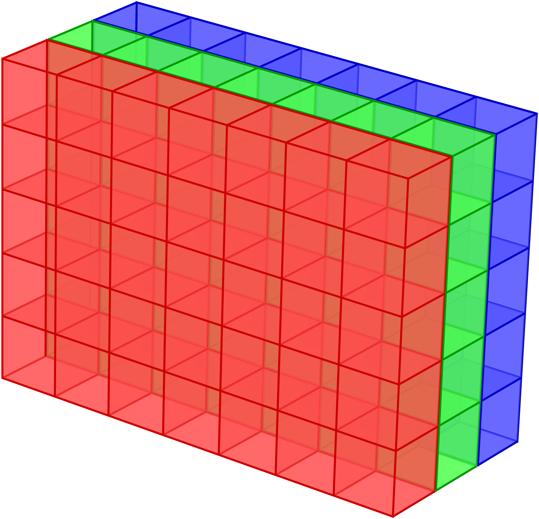
Figure 4.1 The data of a digital colour image composed of \(N\times M\) pixels can be represented as a \(N\times M\times 3\) array where the three planes correspond to the red, green, and blue channels.

The first question to address is how one can store such data structures in Python and how can one make sure that the data can be processed fast. Among the standard datatypes available in Python, a natural candidate would be lists. In Python, lists are very flexible objects which allow to store element of all kinds of datatypes including lists. While this offers us in principle the possibility to represent multi-dimensional data, the flexibility comes with a significant computational overhead. As we will see later, homogeneous data can be handled more efficiently. Leaving the question of efficiency aside for a moment, we can ask whether list are suited at all to represent matrices.

Let us consider a two-dimensional matrix

\[\begin{split}\mathsf{M} = \begin{pmatrix} 1.1 & 2.2 & 3.3\\ 4.4 & 5.5 & 6.6\\ 7.7 & 8.8 & 9.9\end{pmatrix}\,.\end{split}\]

It seems natural to store these data in a list of lists

>>> matrix = [[1.1, 2.2, 3.3], [4.4, 5.5, 6.6], [7.7, 8.8, 9.9]]

of which a single element can be accessed by first selecting the appropriate row and then the desired entry

>>> matrix[0]
[1.1, 2.2, 3.3]
>>> matrix[0][2]
3.3

The only difference with respect to the common mathematical notation is that the indices start at 0 and not at 1. In order to access a single row in a way which makes the two-dimensional character of the matrix more transparent, we could use

>>> matrix[0][:]
[1.1, 2.2, 3.3]

But does this also work for a column? Let us give it a try.

>>> matrix[:][0]
[1.1, 2.2, 3.3]
>>> matrix[:]
[[1.1, 2.2, 3.3], [4.4, 5.5, 6.6], [7.7, 8.8, 9.9]]

The result is rather disappointing because interchanging the two slices yields again the first row. The reason can be seen from the lower two lines. In the first step, we obtain again the full list and in the second step we access its first element, i.e. the first row, not the first column. Even though there are ways to extract a column from a list of lists, e.g. by means of a list comprehension, there is now consistent approach to extracting rows and columns from a list of lists. Our construction is certainly not a good one and we are in need of a new datatype.

4.2.2. NumPy arrays

The new datatype provided by NumPy is a multidimensional homogeneous array of fixed-size items called ndarray. Before starting to explore this datatype, we need to import the NumPy package. While there are different ways to do so, there is one recommended way. Let us take a look at the various alternatives:

from numpy import *                # don't do this!
from numpy import array, sin, cos  # not recommended
import numpy                       # ok, but the following line is better
import numpy as np                 # recommended way

Importing the complete namespace of NumPy as done in the first line is no good idea because the namespace is rather large. Therefore, there is a danger of name conflicts and loss of control. As an alternative, one could restrict the import to the functions actually needed as shown in the second line. However, as can be seen in our example, there exist functions like sine (sin) and cosine (cos) in NumPy. In the body of the code it might not always be evident whether these functions are taken from NumPy or rather the math or cmath module. It is better to more explicit. The import given in the third line is acceptable but it requires to put numpy. in front of each object taken from the NumPy namespace. The usual way to import NumPy is given in the fourth line. Virtually every user seeing np. in the code will assume that the corresponding object belongs to NumPy. It is always a good idea to stick to such conventions to render the code easily understandable.

As the next step, we need to create an array and fill it with data. Whenever we are simply referring to an array, we actually mean an object of datatype ndarray. Given certain similarities with Python lists, it is tempting to use the append method for that purpose as one often does with lists. In fact, NumPy provides an append method. However, because Python lists and NumPy arrays are conceptually quite different, there exist good reasons for avoiding this method if at all possible.

The objects contained in a Python list are typically scattered in memory and the position of each chunk of data is stored in a list of pointers. In contrast, the data of a NumPy array are stored in one contiguous piece of memory. As we will see later, this way of storing an array allows to determine by means of a simple calculation where a certain element can be found. Accessing elements therefore is very efficient.

When appending data to an array, there will generally be no place for the data in memory to guarantee the array to remain contiguous. Appending data in NumPy thus implies the creation of an entirely new array. As a consequence, the data constituting the original array have to be moved to a new place in memory. The time required for this process can become significant for larger arrays and ultimately is limited by the hardware. Using the append method can thus become a serious performance problem.

Generally, when working with NumPy arrays, it is a good idea to avoid the creation of new arrays as much as possible as this may drastically degrade performance. In particular, one should not count on changing the size of an array during the calculation. Already for the creation of the array one should decide how large it will need to be.

One way to find out how a NumPy array can be created it to search the NumPy documentation. This can be done even within Python:

>>> np.lookfor('create array')
Search results for 'create array'
---------------------------------
numpy.array
    Create an array.
numpy.memmap
    Create a memory-map to an array stored in a *binary* file on disk.
numpy.diagflat
    Create a two-dimensional array with the flattened input as a diagonal.
numpy.fromiter
    Create a new 1-dimensional array from an iterable object.
numpy.partition
    Return a partitioned copy of an array.

Here, we have only have reproduced a small part of the output. Furthermore, here and in the following, we assume that NumPy has been imported in the way recommended above so that its namespace can be accessed via the abbreviation np.

Already the first entry in the list of proposed methods is the one to use in our present situation. More information can be obtained as usual by means of help(np.array) or alternatively by

>>> np.info(np.array)
array(object, dtype=None, copy=True, order='K', subok=False, ndmin=0)

Create an array.

Parameters
----------
object : array_like
    An array, any object exposing the array interface, an object whose
    __array__ method returns an array, or any (nested) sequence.
dtype : data-type, optional
    The desired data-type for the array.  If not given, then the type will
    be determined as the minimum type required to hold the objects in the
    sequence.  This argument can only be used to 'upcast' the array.  For
    downcasting, use the .astype(t) method.

Again, only the first part of the output has been reproduced. It is recommended though to take a look at the rest of the help text as it provides a nice example how doctests can be used both for documentation purposes and for testing.

As can be seen from the help text, we need at least one argument object which should be an object with an __array__ method or a possibly nested sequence. Let us consider a first example:

>>> matrix = [[0, 1, 2],
...           [3, 4, 5],
...           [6, 7, 8]]
>>> myarray = np.array(matrix)
>>> myarray
array([[0, 1, 2],
       [3, 4, 5],
       [6, 7, 8]])
>>> type(myarray)
<class 'numpy.ndarray'>

We have started with a list of lists which is a valid argument for np.array. Printing out the result indicates indeed that we have obtained a NumPy array. A confirmation is obtained by asking for the type of myarray.

The data of an array are stored contiguously in memory but what does that really mean for the two-dimensional array which we have just created? Natural ways would be store the date columnwise or rowwise. The first variant is realized in the programming language C while the second variant is used by Fortran. Apart from the actual data, an array obviously needs a number of metadata in order to know how to interpret the content of the memory space attributed to the area. These metadata are a powerful concept because they make it possible to change the interpretation of the data without copying them, thereby contributing to the efficiency of NumPy arrays.

It is useful to get some basic insight into how a NumPy array works. In order to analyze the metadata, we use a short function enabling us to list the attributes of an array.

def array_attributes(a):
    for attr in ('ndim', 'size', 'itemsize', 'dtype', 'shape', 'strides'):
        print(f'{attr:8s}: {getattr(a, attr)}')

A convenient way of generating an array for test purposes is the arange function which works very much like the standard range iterator as far as its basic arguments start, stop, and step are concerned. In this way, we can easily construct a one-dimensional array with integer entries from 0 to 15 and inspect its properties:

>>> matrix = np.arange(16)
>>> matrix
array([ 0,  1,  2,  3,  4,  5,  6,  7,  8,  9, 10, 11, 12, 13, 14, 15])
>>> array_attributes(matrix)
ndim    : 1
size    : 16
itemsize: 8
dtype   : int64
shape   : (16,)
strides : (8,)

Let us take a look at the different attributes. The attribute ndim indicates the number of dimension of the array which in our example is one-dimensional and therefore ndim equals 1. The size of 16 means that the array contains a total of 16 items. Each item has an itemsize of 8 bytes or 64 bits, resulting in a total size of 128 bytes:

>>> matrix.nbytes
128

The attribute dtype represents the datatype which in our example is int64, i.e. an integer type of a length of 64 bits. Quite in contrast to the usual integer type in Python which can in principle handle integers of arbitrary size, the integer values in our array are clearly limited. An example using integers of only 8 bits length can serve to illustrate the problem of overflows:

>>> np.arange(1, 160, 10, dtype=np.int8)
array([   1,   11,   21,   31,   41,   51,   61,   71,   81,   91,  101,
        111,  121, -125, -115, -105], dtype=int8)

Take a look at the items in this array and try to understand what is going on.

>>> for k, v in np.core.numerictypes.sctypes.items():
...     print(k)
...     for elem in v:
...         print(f'    {elem}')
...
int
    <class 'numpy.int8'>
    <class 'numpy.int16'>
    <class 'numpy.int32'>
    <class 'numpy.int64'>
uint
    <class 'numpy.uint8'>
    <class 'numpy.uint16'>
    <class 'numpy.uint32'>
    <class 'numpy.uint64'>
float
    <class 'numpy.float16'>
    <class 'numpy.float32'>
    <class 'numpy.float64'>
    <class 'numpy.float128'>
complex
    <class 'numpy.complex64'>
    <class 'numpy.complex128'>
    <class 'numpy.complex256'>
others
    <class 'bool'>
    <class 'object'>
    <class 'bytes'>
    <class 'str'>
    <class 'numpy.void'>

The first four groups of datatypes include integers, unsigned integers, floats and complex numbers of different sizes. Among the other types, booleans as well as strings are of some interest. Note, however, that the data in an array always should be homogeneous. If different datatypes are mixed in the assignment to an array, it may happen that a datatype is cast to a more flexible one. For strings, the size of each entry will be determined by the longest string.

Probably the most interesting attributes of an array are shape and strides because the allow us to reinterpret the data of the original one-dimensional array in different ways without the need to copy from memory to memory. Let us first try to understand the meaning of the tuples (16,) for shape and (8,) for strides. Both tuples have the same size which equals one because the considered array is one-dimensional. Therefore, shape does not contain any new information. It simply reflects the size of the array as does the attribute size. The value of strides means that in order to move from the beginning of an item in memory to the beginning of the next one, one needs to more eight bytes. This information is consistent with the itemsize. What seems like redundant information becomes more interesting when we go from a one-dimensional array to a multi-dimensional array. For simplicity we convert the our one-dimensional array matrix into a two-dimensional square array. To this purpose we make use of the reshape method:

>>> matrix = matrix.reshape(4, 4)
>>> matrix
array([[ 0,  1,  2,  3],
       [ 4,  5,  6,  7],
       [ 8,  9, 10, 11],
       [12, 13, 14, 15]])
>>> array_attributes(matrix)
ndim    : 2
size    : 16
itemsize: 8
dtype   : int64
shape   : (4, 4)
strides : (32, 8)

In the first line, we bring our one-dimensional array with 16 elements into a \(4\times4\) array. Three attributes change their value in this process. ndim is now 2 because we created a two-dimensional array. The shape attribute with value (4, 4) reflects the fact that now we have 4 rows and 4 columns. Finally, the strides are given by the tuple (32, 8). To go in memory from an item to the item in the next column and in the same row means that we should move by 8 bytes. The two items are neighbors in memory. However, if we stay within the same column and want to move to the next row, we have to jump by 32 bytes in memory.

To further illustrate the meaning of shape and strides we consider a second example. A linear arrangement of six data in memory can be interpreted in three different ways as depicted in Figure 4.2. In the uppermost example, strides is set to (8,). The tuple strides tuple contains only one element and we are therefore dealing with a one-dimensional array. Assuming the datasize to be 8, the array consists of all six data elements. In the second case, strides are set to (24, 8). Accordingly, the matrix consists of two rows and three columns. Finally, in the bottom example with strides equal to (16, 8), the data are interpreted as a matrix consisting of two columns and three rows. Note that no rearrangement of data in memory is required in order to go from one matrix to another one. Only the way, how the position of a certain element in memory is obtained, changes when strides is modified.

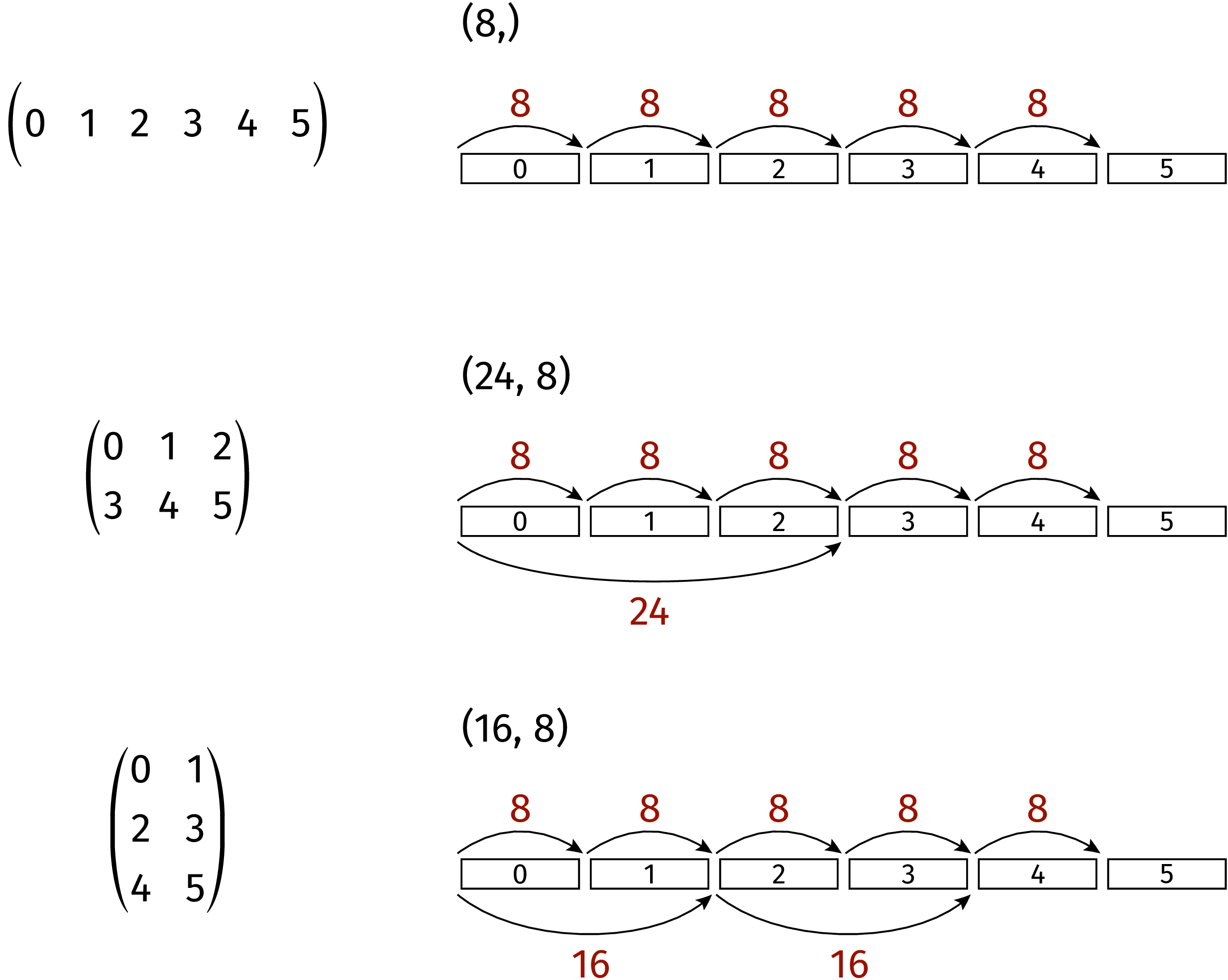
Figure 4.2 Linear data in memory can be interpreted in different ways by appropriately choosing the strides tuple.

A two-dimensional matrix can easily be transposed. Behind the scenes the values in the strides tuple are interchanged:

>>> a = np.arange(9).reshape(3, 3)
>>> a
array([[0, 1, 2],
       [3, 4, 5],
       [6, 7, 8]])
>>> a.strides
(24, 8)
>>> a.T
array([[0, 3, 6],
       [1, 4, 7],
       [2, 5, 8]])
>>> a.T.strides
(8, 24)

Strides are a powerful concept. However, one should be careful not to violate the boundaries of the data because otherwise memory might be interpreted in a meaningless way. In the following two examples, the first demonstrates an interesting way to create a special pattern of data. The second example, where one of the strides is only half of the datasize, shows how useless results can be produced:

>>> a = np.arange(16).reshape(4, 4)
>>> a
array([[ 0,  1,  2,  3],
       [ 4,  5,  6,  7],
       [ 8,  9, 10, 11],
       [12, 13, 14, 15]])
>>> a.strides = (8, 8)
>>> a
array([[0, 1, 2, 3],
       [1, 2, 3, 4],
       [2, 3, 4, 5],
       [3, 4, 5, 6]])
>>> a.strides = (8, 4)
>>> a
array([[          0,  4294967296,           1,  8589934592],
       [          1,  8589934592,           2, 12884901888],
       [          2, 12884901888,           3, 17179869184],
       [          3, 17179869184,           4, 21474836480]])

In the end, the user manipulating strides is responsible for all consequences which his or her action may have.

4.2.3. Creating arrays

We have seen in the previous section that an array can be created by providing np.array with an object possessing an __array__ method or a nested sequence. However, this requires to create the object or nested sequence in the first place. Often, more convenient methods exist. As we have pointed out earlier, when creating an array, one should have an idea of the desired size and usually also of the datatype to be stored in the array. Given this information, there exists a variety of methods to create an array depending on the specific needs.

It is not unusual to start with an array filled with zeros. Let us create a \(2\times2\) array:

>>> a = np.zeros((2, 2))
>>> a
array([[0., 0.],
       [0., 0.]])
>>> a.dtype
dtype('float64')

As we can see, the default type is float64. If we prefer an array of integers, we could specify the dtype:

>>> a = np.zeros((2, 2), dtype=np.int)
>>> a
array([[0, 0],
       [0, 0]])
>>> a.dtype
dtype('int64')

As an alternative, one can create an empty array which should however not be confused with an array filled with zeros. An empty array will just claim the necessary amount of memory without doing anything to the data present in that piece of memory. This is fine if one is going to specify the content of all array data subsequently before using the array. Otherwise, one will deal with random data:

>>> np.empty((3, 3))
array([[6.94870988e-310, 6.94870988e-310, 7.89614591e+150],
       [1.37038197e-013, 2.08399685e+064, 3.51988759e+016],
       [8.23900250e+015, 7.32845376e+025, 1.71130458e+059]])

An alternative to filling an array with zeros could be to fill it with ones or another value which can be obtained by multiplication:

>>> np.ones((2, 2))
array([[1., 1.],
       [1., 1.]])
>>> 10*np.ones((2, 2))
array([[10., 10.],
       [10., 10.]])

As one can see in this example, the multiplication by a number acts on all elements of the array. This behavior is probably what one would expect at this point. As we will see in Section 4.2.5, we are here making use of a more general concept referred to as broadcasting.

Often, one needs arrays with more structure than the one we have created so far. It is not uncommon, that the diagonal entries take a special form. An identity matrix can easily be created:

>>> np.identity(3)
array([[1., 0., 0.],
       [0., 1., 0.],
       [0., 0., 1.]])

The result will always be a square matrix. A more general method to fill the diagonal or a shifted diagonal is provided by np.eye:

>>> np.eye(2, 4)
array([[1., 0., 0., 0.],
       [0., 1., 0., 0.]])
>>> np.eye(4, k=1)
array([[0., 1., 0., 0.],
       [0., 0., 1., 0.],
       [0., 0., 0., 1.],
       [0., 0., 0., 0.]])
>>> 2*np.eye(4)-np.eye(4, k=1)-np.eye(4, k=-1)
array([[ 2., -1.,  0.,  0.],
       [-1.,  2., -1.,  0.],
       [ 0., -1.,  2., -1.],
       [ 0.,  0., -1.,  2.]])

These examples show that np.eye does not expect a tuple specifying the shape. Instead, the first two arguments give the number of rows and columns. If the second argument is absent, the resulting matrix is a square matrix. In the second and third example, the missing second argument is the reason why we have to specify that the second argument is intended as the shift k of the diagonal. The third example gives an idea of how the Hamiltonian for the kinetic energy in a tight-binding model can be constructed.

It is also possible to generate diagonals or, by specifying k, shifted diagonals with different values:

>>> np.diag([1, 2, 3, 4])
array([[1, 0, 0, 0],
       [0, 2, 0, 0],
       [0, 0, 3, 0],
       [0, 0, 0, 4]])

Using a two-dimensional array as argument, its diagonal elements can be extracted by means of the same function:

>>> matrix = np.arange(16).reshape(4, 4)
>>> matrix
array([[ 0,  1,  2,  3],
       [ 4,  5,  6,  7],
       [ 8,  9, 10, 11],
       [12, 13, 14, 15]])
>>> np.diag(matrix)
array([ 0,  5, 10, 15])

If the elements of an array can be expressed as a function of the indices, fromfunction can be used to generate the elements. As a simple example, we create a multiplication table:

>>> np.fromfunction(lambda i, j: (i+1)*(j+1), shape=(6, 6), dtype=np.int)
array([[ 1,  2,  3,  4,  5,  6],
       [ 2,  4,  6,  8, 10, 12],
       [ 3,  6,  9, 12, 15, 18],
       [ 4,  8, 12, 16, 20, 24],
       [ 5, 10, 15, 20, 25, 30],
       [ 6, 12, 18, 24, 30, 36]])

Even though we present a two-dimensional example, the latter approach can be used to create arrays of an arbitrary dimension.

The function used in the previous example was a very simple one. Occasionally, one might need more complicated functions like one of the trigonometric functions. In fact, NumPy provides a number of so-called universal functions which we will discuss in Section 4.2.6. Such functions accept an array as argument and return an array. Here, we will concentrate on creating arguments for universal functions.

A first function is arange which we have used before for integers. It is a generalization of the standard range which works even for floats:

>>> np.arange(1, 2, 0.1)
array([1. , 1.1, 1.2, 1.3, 1.4, 1.5, 1.6, 1.7, 1.8, 1.9])

As with range, the first argument is the start value while the second argument refers to the final value which is not included. Because of rounding errors, the last statement is not always true. Finally, the third argument is the stepwidth. An alternative is offered by the linspace function which by default will make sure that the start value and the final value are part of the array. Instead of the stepwidth, the number of points is specified:

>>> np.linspace(1, 2, 11)
array([1. , 1.1, 1.2, 1.3, 1.4, 1.5, 1.6, 1.7, 1.8, 1.9, 2. ])

A common mistake is to assume that the last argument gives the number of intervals which, however, is not the case. Thus, there is some danger that one is off by one in the last argument. Sometimes it is useful to ask for the stepwidth:

>>> np.linspace(1, 4, 7, retstep=True)
(array([1. , 1.5, 2. , 2.5, 3. , 3.5, 4. ]), 0.5)

Here, the stepwidth does not need to be determined by hand.

Occasionally, a logarithmic scale can be useful. In this case, the start value and the final value refer to the exponent. The base by default is ten but can be modified, if necessary:

>>> np.logspace(0, 3, 4)
array([   1.,   10.,  100., 1000.])
>>> np.logspace(0, 2, 5, base=2)
array([1.        , 1.41421356, 2.        , 2.82842712, 4.        ])

The following example illustrate the application of linspace in a universal function to produce a graphical representation of the function:

>>> import matplotlib.pyplot as plt
>>> x = np.linspace(0, 2*np.pi, 100)
>>> y = np.sin(x)
>>> plt.plot(x, y)
[<matplotlib.lines.Line2D object at 0x7f22d619cc88>]

The generated graph is reproduced in Figure 4.3.

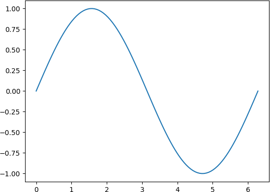
Figure 4.3 Simple example of a function graph generated by operating with a universal function on an array generated by linspace.

Arrays can also be filled with data taken from a file. This can for example be the case if data obtained from a measurement are first stored in a file before being processed or if numerical data are stored before a graphical representation is produced. Assume that we have a data file called mydata.dat with the following content:

# time position
   0.0   0.0
   0.1   0.1
   0.2   0.4
   0.3   0.9

Loading the data from the file, we obtain:

>>> np.loadtxt('mydata.dat')
array([[0. , 0. ],
       [0.1, 0.1],
       [0.2, 0.4],
       [0.3, 0.9]])

By default, lines starting with # will be considered as comments and are ignored. The function loadtxt offers a number of arguments to load data in a rather flexible way. Even more possibilities are offered by genfromtxt which is also able to deal with missing values. See the documentation of loadtxt and genfromtxt for more information.

In numerical simulations, it is often necessary to generate random numbers and if many of them are needed, it may be efficient to generate an array filled with random numbers. While NumPy offers many different distributions of random numbers, we concentrate on equally distributed random numbers in an interval from 0 to 1. An array of a given shape filled with such random numbers can be obtained as follows:

>>> np.random.rand(2, 5)
array([[0.76455979, 0.09264023, 0.47090143, 0.81327348, 0.42954314],
       [0.37729755, 0.20315983, 0.62982297, 0.0925838 , 0.37648008]])
>>> np.random.rand(2, 5)
array([[0.23714395, 0.22286043, 0.97736324, 0.19221663, 0.18420108],
       [0.14151036, 0.07817544, 0.4896872 , 0.90010128, 0.21834491]])

Clearly, the set of random numbers changes at each call to random.rand. Occasionally, one would like to have reproducible random numbers, for example during unit tests or to reproduce a particularly interesting scenario in a simulation. Then one can set a seed:

>>> np.random.seed(123456)
>>> np.random.rand(2, 5)
array([[0.12696983, 0.96671784, 0.26047601, 0.89723652, 0.37674972],
       [0.33622174, 0.45137647, 0.84025508, 0.12310214, 0.5430262 ]])
>>> np.random.seed(123456)
>>> np.random.rand(2, 5)
array([[0.12696983, 0.96671784, 0.26047601, 0.89723652, 0.37674972],
       [0.33622174, 0.45137647, 0.84025508, 0.12310214, 0.5430262 ]])

Sometimes, it is convenient to graphically represent the matrix elements. Figure 4.4 shows an example generated by the following code:

>>> import matplotlib.pyplot as plt
>>> np.random.seed(42)
>>> data = np.random.rand(20, 20)
>>> plt.imshow(data, cmap=plt.cm.hot, interpolation='none')
<matplotlib.image.AxesImage object at 0x7f39027afe48>
>>> plt.colorbar()
<matplotlib.colorbar.Colorbar object at 0x7f39027e58d0>
>>> plt.show()

Not that the argument interpolation of plt.imshow is set to 'none' to ensure that no interpolation is done which might blur the image.

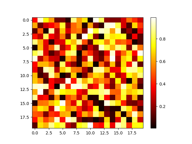
Figure 4.4 Graphical representation of an array filled with random numbers.

4.2.4. Indexing arrays

One way of accessing sets of elements of an array makes use of slices which we know from Python lists. A slice is characterized by a start index, a stop index whose corresponding element is excluded, and step which indicates the stepsize. Negative indices are counted from the end of the corresponding array dimension and a negative value of step implies walking in the direction of decreasing indices.

We start by a few examples of slicing for a one-dimensional array:

>>> a = np.arange(10)
>>> a
array([0, 1, 2, 3, 4, 5, 6, 7, 8, 9])
>>> a[:]
array([0, 1, 2, 3, 4, 5, 6, 7, 8, 9])
>>> a[1:4]
array([1, 2, 3])
>>> a[5:-2]
array([5, 6, 7])
>>> a[::2]
array([0, 2, 4, 6, 8])
>>> a[1::2]
array([1, 3, 5, 7, 9])
>>> a[::-1]
array([9, 8, 7, 6, 5, 4, 3, 2, 1, 0])

The third input, i.e. a[:] leaves the start and stop values open so that all array elements are returned because by default step equals 1. In the next example, we recall that indices in an array as in a list start at 0. Therefore, we obtain the second up to the fourth element of the array. In the fifth input, the second element counted from the end of the array is not part of the result so that we obtain the numbers from 5 to 7. We could have used a[5:8] instead. In the sixth input, start and stop values are again left open, so that the resulting array starts with 0 but then proceeds in steps of 2 according to the value of step given. In the following example, start is set to 1 and we obtain the elements left out in the previous example. The last example inverts the sequence of array elements by specifying a step of -1.

The use of a[:] deserves a bit more attention. In the case of a list, it would yield a shallow copy of the original list. For an array, the behavior is somewhat different. Let us first consider an alias:

>>> b = a
>>> b
array([0, 1, 2, 3, 4, 5, 6, 7, 8, 9])
>>> id(a), id(b)
(140493158678656, 140493158678656)
>>> b[0] = 42
>>> a
array([42,  1,  2,  3,  4,  5,  6,  7,  8,  9])

In this case, b is simply an alias for a and refers to the same object. A modification of elements of b will also be visible in a. Now, let us consider a slice comprising all elements:

>>> a = np.arange(10)
>>> b = a[:]
>>> b
array([0, 1, 2, 3, 4, 5, 6, 7, 8, 9])
>>> id(a), id(b)
(140493155003008, 140493155003168)
>>> b[0] = 42
>>> a
array([42,  1,  2,  3,  4,  5,  6,  7,  8,  9])

Now a new object is generated, but it refers to the same piece of memory. A modification of elements in b will still be visible in a. In order to really obtain a copy of an array, one applies the copy function:

>>> a = np.arange(10)
>>> b = np.copy(a)
>>> b[0] = 42
>>> a
array([0, 1, 2, 3, 4, 5, 6, 7, 8, 9])
>>> b
array([42,  1,  2,  3,  4,  5,  6,  7,  8,  9])

It is rather straightforward to extend the concept of slicing to higher dimensions and we again go through a number of examples to illustrate the idea. Note that in no case a new array is created in memory so that slicing is an efficient way of extracting a certain subset of array elements. Our base array is:

>>> a = np.arange(36).reshape(6, 6)
>>> a
array([[ 0,  1,  2,  3,  4,  5],
       [ 6,  7,  8,  9, 10, 11],
       [12, 13, 14, 15, 16, 17],
       [18, 19, 20, 21, 22, 23],
       [24, 25, 26, 27, 28, 29],
       [30, 31, 32, 33, 34, 35]])

In view of the two dimensions, we now need two slices separated by a comma, the first one for the rows and the second one for the columns. The full array is thus recovered by:

>>> a[:, :]
array([[ 0,  1,  2,  3,  4,  5],
       [ 6,  7,  8,  9, 10, 11],
       [12, 13, 14, 15, 16, 17],
       [18, 19, 20, 21, 22, 23],
       [24, 25, 26, 27, 28, 29],
       [30, 31, 32, 33, 34, 35]])

A sub-block can be extracted as follows:

>>> a[2:4, 3:6]
array([[15, 16, 17],
       [21, 22, 23]])

As already mentioned, the first slice pertains to the rows, so that we choose elements from the third and fourth row. The second slice refers to columns four to six so that we indeed end up with the output reproduced above.

Sub-blocks do not need to be contiguous. We can even choose different values for step in different dimensions:

>>> a[::2, ::3]
array([[ 0,  3],
       [12, 15],
       [24, 27]])

In this example, we have selected every second row and every third column. If we want to start with the third row, we could write:

>>> a[2::2, ::3]
array([[12, 15],
       [24, 27]])

The following example illustrates a case where only one slice is specified:

>>> a[2:4]
array([[12, 13, 14, 15, 16, 17],
       [18, 19, 20, 21, 22, 23]])

The first slice still applies to the row and the missing second slice is replaced by default by :: representing all columns.

The interpretation of the last example requires to make connection between the axis number and its meaning in terms of the array elements. In a two-dimensional array, the position of the indices follows the convention used in mathematics as shown in Figure 4.5. This correctness of this interpretation can also be verified by means of operations which can act along a single axis as is the case for sum:

>>> a.sum(axis=0)
array([ 90,  96, 102, 108, 114, 120])
>>> a.sum(axis=1)
array([ 15,  51,  87, 123, 159, 195])
>>> a.sum()
630

In the first case, the summation is performed along the columns while in the second case the elements in a given row are added. If no axis is specified, all array elements are summed.

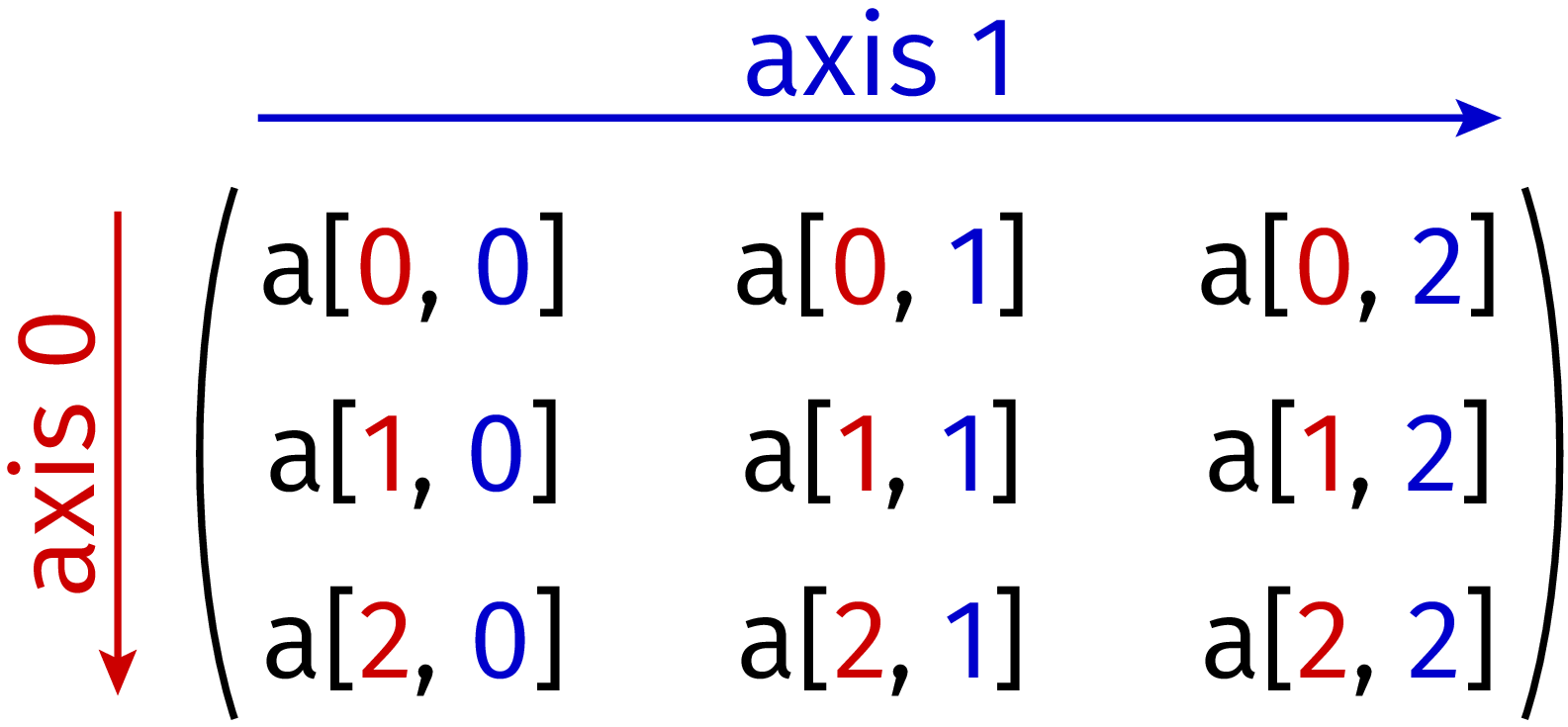
Figure 4.5 In a two-dimensional array, the first index corresponding to axes 0 denotes the row while the second index corresponding to axes 1 denotes the column. This convention is consistent with the one used in mathematics.

We illustrate the generalization to higher dimensions by considering a three-dimensional array:

>>> b = np.arange(24).reshape(2, 3, 4)
>>> b
array([[[ 0,  1,  2,  3],
        [ 4,  5,  6,  7],
        [ 8,  9, 10, 11]],

       [[12, 13, 14, 15],
        [16, 17, 18, 19],
        [20, 21, 22, 23]]])

Interpreting the array in terms of nested lists, the outer level contains two two-dimensional arrays along axis 0 as displayed in Figure 4.6. Within the two-dimensional arrays, the outer level corresponds to axis 1 and the innermost level corresponds to axis 2.

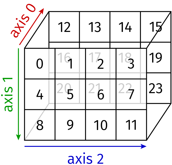
Figure 4.6 A three-dimensional array with its three axes.

Cutting along the three axes, we obtain the following two-dimensional arrays:

>>> b[0]
array([[ 0,  1,  2,  3],
       [ 4,  5,  6,  7],
       [ 8,  9, 10, 11]])
>>> b[:, 0]
array([[ 0,  1,  2,  3],
       [12, 13, 14, 15]])
>>> b[:, :, 0]
array([[ 0,  4,  8],
       [12, 16, 20]])

These three arrays correspond to the front plane along axis 0, the upper plane along axis 1 and the left-most plane along axis 2, respectively. In the last example, an appropriate number of colons can simply be replaced by an ellipsis:

>>> b[..., 0]
array([[ 0,  4,  8],
       [12, 16, 20]])

In order to make the meaning of this notation unique, only one ellipsis is permitted, but it may appear even between indices like in the following example:

>>> c = np.arange(16).reshape(2, 2, 2, 2)
>>> c
array([[[[ 0,  1],
         [ 2,  3]],

        [[ 4,  5],
         [ 6,  7]]],


       [[[ 8,  9],
         [10, 11]],

        [[12, 13],
         [14, 15]]]])
>>> c[0, ..., 0]
array([[0, 2],
       [4, 6]])

When selecting a column in a two-dimensional array, one in principle has two ways to do so. However, they are leading to different results:

>>> a[:, 0:1]
array([[ 0],
       [ 6],
       [12],
       [18],
       [24],
       [30]])
>>> a[:, 0]
array([ 0,  6, 12, 18, 24, 30])

In the first case, a two-dimensional array is produced where the second dimension happens to be of length 1. In the second case, the first column is explicitly selected and one ends up with a one-dimensional array. This example may lead to the question whether there is a way to convert a one-dimensional array into a two-dimensional array containing one column or one row. Such a conversion may be necessary in the context of broadcasting which we will discuss in Section 4.2.5. The following example demonstrates how the dimension of an array can be increased by means of a newaxis:

>>> d = np.arange(4)
>>> d
array([0, 1, 2, 3])
>>> d[:, np.newaxis]
array([[0],
       [1],
       [2],
       [3]])
>>> d[:, np.newaxis].shape
(4, 1)
>>> d[np.newaxis, :]
array([[0, 1, 2, 3]])
>>> d[np.newaxis, :].shape
(1, 4)

So far, we have selected subsets of array elements by means of slicing. Another option is the so-called fancy indexing where elements are specified by lists or arrays of integers or Booleans for each dimension of the array. Let us consider a few examples:

>>> a
array([[ 0,  1,  2,  3,  4,  5],
       [ 6,  7,  8,  9, 10, 11],
       [12, 13, 14, 15, 16, 17],
       [18, 19, 20, 21, 22, 23],
       [24, 25, 26, 27, 28, 29],
       [30, 31, 32, 33, 34, 35]])
>>> a[[0, 2, 1], [1, 3, 5]]
array([ 1, 15, 11])

The lists for axes 0 and 1 combine to yield the index pairs of the elements to be selected. In our example, these are a[0, 1], a[2, 3], and a[1, 5]. As this example shows, the indices in one list do not need to increase. They rather have be to chosen as a function of the elements which shall be selected. In this example, there is no way how the two-dimensional form of the original array can be maintained and we simply obtain a one-dimensional array containing the three elements selected by the two lists.

A two-dimensional array can be obtained from an originally two-dimensional array if entire rows or columns are selected like in the following example:

>>> a[:, [0, 3, 5]]
array([[ 0,  3,  5],
       [ 6,  9, 11],
       [12, 15, 17],
       [18, 21, 23],
       [24, 27, 29],
       [30, 33, 35]])

Here, we have only specified a list for axis 1 and chosen entire columns. Note that the chosen columns are not equidistant and thus cannot be obtained by slicing.

Our last example uses fancy indexing with a boolean array. We create an array of random numbers and want to set all entries smaller than 0.5 to zero. After creating an array of random numbers from which we construct a Boolean area by comparing with 0.5. The resulting array is then used not to extract array elements but to set selected array elements to zero:

>>> randomarray = np.random.rand(10)
>>> randomarray
array([0.48644931, 0.13579493, 0.91986082, 0.38554513, 0.38398479,
       0.61285717, 0.60428045, 0.01715505, 0.44574082, 0.85642709])
>>> indexarray = randomarray < 0.5
>>> indexarray
array([ True,  True, False,  True,  True, False, False,  True,  True,
       False])
>>> randomarray[indexarray] = 0
>>> randomarray
array([0.        , 0.        , 0.91986082, 0.        , 0.        ,
       0.61285717, 0.60428045, 0.        , 0.        , 0.85642709])

If instead of setting values below 0.5 to zero, we would have wanted to set them to 0.5, we could have avoided fancy indexing by using np.clip.

As an application of slicing and fancy indexing, we consider a NumPy implementation of the sieve of Eratosthenes to determine prime numbers. The principle is illustrated in Figure 4.7 where the steps required to determine all prime numbers below 50 are depicted. We start out with a list of integers up to 49. It is convenient to include 0 to be consistent with the fact that indexing starts at 0 in NumPy. A corresponding array is_prime is initialized with the Boolean value True. In each iteration numbers found not be prime have their value set to False. Initially, we mark 0 and 1 as non-primes.

Now we iterate through the array and consider successively each prime number which we can find. The first one will be 2. Clearly, all multiples of 2 are not prime and we can cross them out. The next prime is 3, but now we can start crossing out multiples of 3 at 9. In general, for a prime number \(p\), we start crossing out multiples of \(p\) at \(p^2\) because all smaller multiples of \(p\) have been crossed out before. The maximum number to be considered as candidate is the largest integer smaller or equal to the maximum integer to be considered. In our example, we consider integers up to 49 and thus the largest candidate is 7 which happens to be prime.

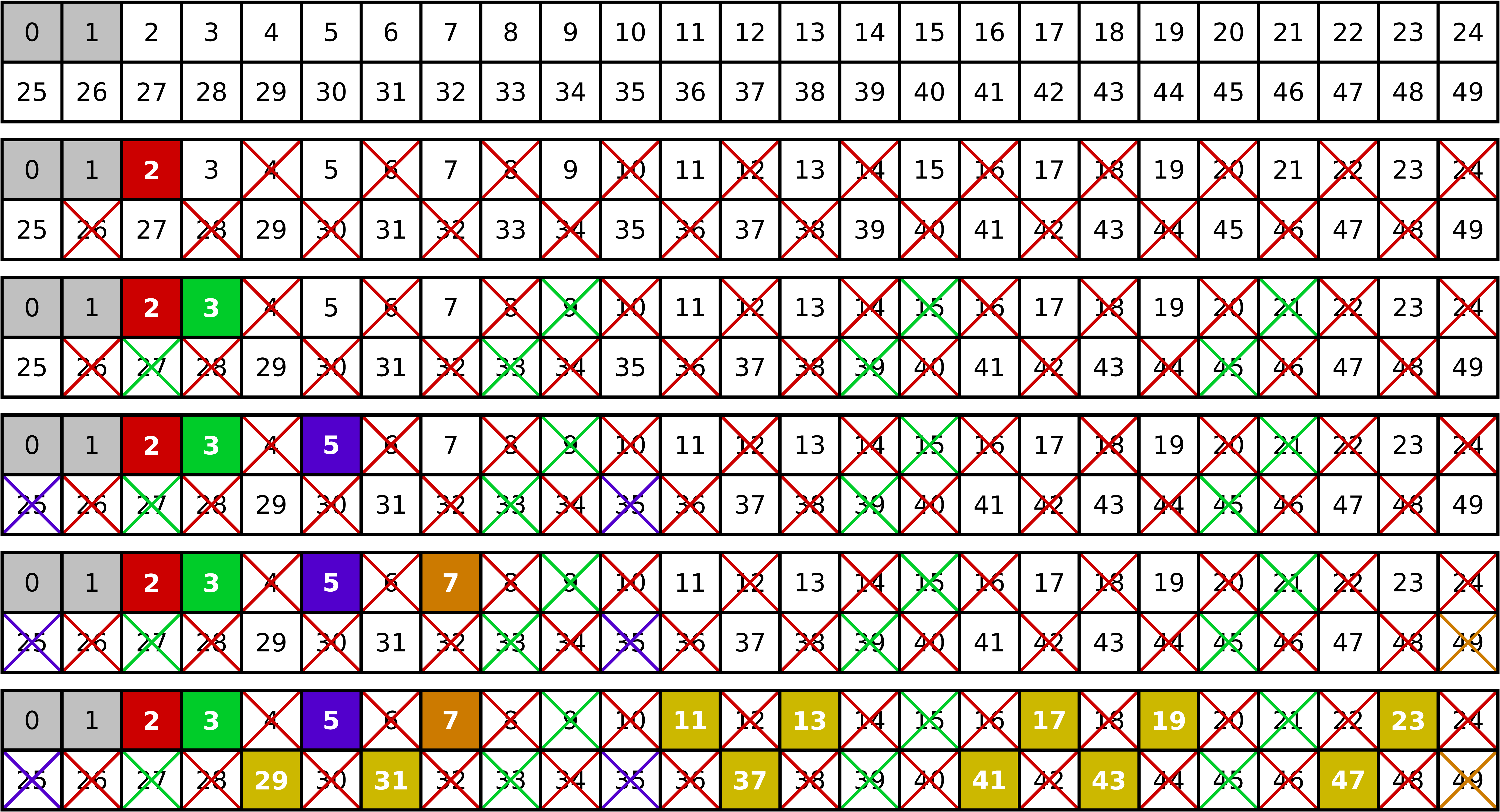
Figure 4.7 Iteration steps when the sieve of Eratosthenes is used to determine the prime numbers below 50. For details see the main text.

This algorithm can be implemented in the following way where we have chosen to print not only the final result but also the intermediate steps.

import math
import numpy as np

nmax = 49
integers = np.arange(nmax+1)
is_prime = np.ones(nmax+1, dtype=bool)
is_prime[:2] = False
for j in range(2, int(math.sqrt(nmax))+1):
    if is_prime[j]:
        is_prime[j*j::j] = False
    print(integers[is_prime])

This script produces the following output:

[ 2  3  5  7  9 11 13 15 17 19 21 23 25 27 29 31 33 35 37 39 41 43 45 47 49]
[ 2  3  5  7 11 13 17 19 23 25 29 31 35 37 41 43 47 49]
[ 2  3  5  7 11 13 17 19 23 25 29 31 35 37 41 43 47 49]
[ 2  3  5  7 11 13 17 19 23 29 31 37 41 43 47 49]
[ 2  3  5  7 11 13 17 19 23 29 31 37 41 43 47 49]
[ 2  3  5  7 11 13 17 19 23 29 31 37 41 43 47]

In line 6 of the Python code, we use np.ones with type bool to mark all entries as potential primes. In line 10, slicing is used to mark all multiples of j starting at the square of j as non-primes. Finally, in line 11, fancy indexing is used. The Boolean array is_prime indicates through the value True which entries in the array integers should be printed.

4.2.5. Broadcasting

In the previous sections, we have seen examples where an operation involved a scalar value and an array. This was the case in Section 4.2.3 where we multiplied an array created by np.ones with a number. Another example appeared in Section 4.2.4 where in our discussion of fancy indexing we compared an array with a single number. Even though NumPy behaved in a perfectly natural way, these examples are special cases of a more general concept, the so-called broadcasting.

An array can be broadcast to a larger array provided the shapes satisfy certain conditions. In order to obtain the same dimension as the one of the target array, dimensions of size 1 are prepended. Then, each component of the shape of the original array has to be equal to the corresponding component of the shape of the target array or the component has to equal 1. In Figure 4.8, the target array has shape (3, 4). The arrays with shapes (1,), (4, ), and (3, 1) satisfy this conditions and can be broadcast as shown in the figure. In contrast, this is not possible for an array of shape (3,) as is demonstrated in the figure. We emphasize the difference between the arrays of shape (3,) and (3, 1).

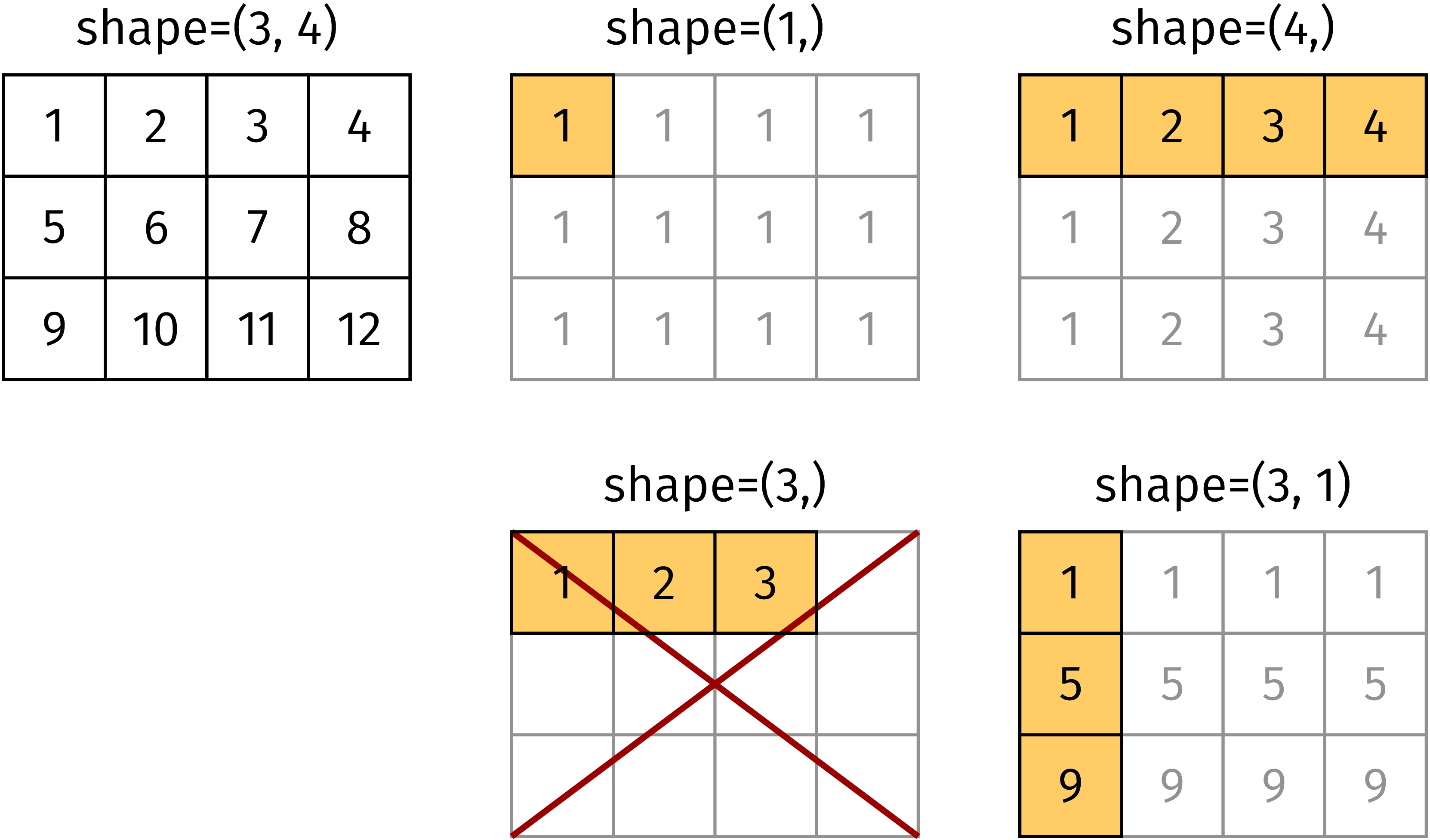
Figure 4.8 For appropriate shapes, the matrix elements in the highlighted cells can be broadcast to create the full shape (3, 4) in this example. An array of shape (3,) cannot be broadcast to shape (3, 4)

As the second image in Figure 4.8 shows, a scalar is broadcast to an array of the desired shape with all elements being equal. Multiplying an array with a scalar, we expect that each array element is multiplied by the scalar. As a consequence, the multiplication of two arrays is carried out element by element. In other words, a matrix multiplication cannot be done by means of the * operator:

>>> a = np.arange(4).reshape(2, 2)
>>> a
array([[0, 1],
       [2, 3]])
>>> b = np.arange(4, 8).reshape(2, 2)
>>> b
array([[4, 5],
       [6, 7]])
>>> a*b
array([[ 0,  5],
       [12, 21]])

The matrix multiplication can be achieved in a number of different ways:

>>> np.dot(a, b)
array([[ 6,  7],
       [26, 31]])
>>> a.dot(b)
array([[ 6,  7],
       [26, 31]])
>>> a @ b
array([[ 6,  7],
       [26, 31]])

The use of the @ operator for the matrix multiplication requires at least Python 3.5 and NumPy 1.10.

4.2.6. Universal functions

The mathematical functions provided by the math and cmath modules from the Python standard library accept only single real or complex values but no arrays. For the latter purpose, NumPy and also the scientific library SciPy offer so-called universal functions:

>>> import math
>>> x = np.linspace(0, 2, 11)
>>> x
array([0. , 0.2, 0.4, 0.6, 0.8, 1. , 1.2, 1.4, 1.6, 1.8, 2. ])
>>> math.sin(x)
Traceback (most recent call last):
  File "<stdin>", line 1, in <module>
TypeError: only size-1 arrays can be converted to Python scalars
>>> np.sin(x)
array([0.        , 0.19866933, 0.38941834, 0.56464247, 0.71735609,
       0.84147098, 0.93203909, 0.98544973, 0.9995736 , 0.97384763,
       0.90929743])

Universal functions can handle multi-dimensional arrays as well:

>>> x = np.array([[0, np.pi/2], [np.pi, 3/2*np.pi]])
>>> x
array([[0.        , 1.57079633],
       [3.14159265, 4.71238898]])
>>> np.sin(x)
array([[ 0.0000000e+00,  1.0000000e+00],
       [ 1.2246468e-16, -1.0000000e+00]])

This example shows that the mathematical constant \(\pi\) is not only available from the math and cmath modules but also from the NumPy package. Many of the functions provided by the math module are available as universal functions in NumPy and NumPy offers a few universal functions not available as normal functions neither in math nor in cmath. Details on the functions provided by NumPy are given in the section on Mathematical functions in the NumPy reference guide.

While the universal functions in NumPy are mostly restricted to the common mathematical functions, special functions are available through the SciPy package. Often but not always, these functions are implemented as universal functions as well. As an example, we create a plot of the Airy function \(\mathrm{Ai}(x)\) appearing e.g. in the theory of the rainbow or the quantum mechanics in a linear potential:

>>> from scipy.special import airy
>>> x = np.linspace(-20, 5, 300)
>>> ai, aip, bi, bip = airy(x)
>>> plt.plot(x, ai, label="Ai(x)")
[<matplotlib.lines.Line2D object at 0x7f62184e2278>]
>>> plt.plot(x, aip, label="Ai'(x)")
[<matplotlib.lines.Line2D object at 0x7f621bbb4518>]
>>> plt.legend()
>>> plt.show()

There exist two types of Airy functions \(\mathrm{Ai}(x)\) and \(\mathrm{Bi}(x)\) which together with their derivatives are calculated by the airy function in one go. The Airy function \(\mathrm{Ai}(x)\) and its derivative are displayed in Figure 4.9.

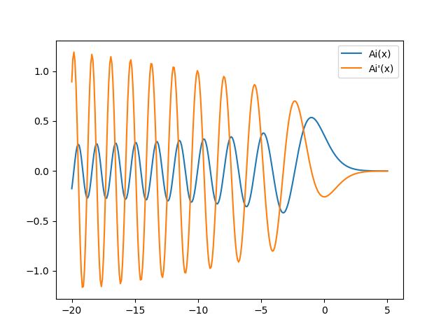
Figure 4.9 Airy function \(\mathrm{Ai}(x)\) and its derivative.

Occasionally, one needs to create a two-dimensional plot of a function of two variables. In order to ensure that the resulting array is two-dimensional, the one-dimensional arrays for the two variables need to run along different axes. A convenient way to do so is the mesh grid. The function mgrid creates two two-dimensional arrays where in one array the values change along the column while in the other array they change along the rows:

>>> np.mgrid[0:2:0.5, 0:1:0.5]
array([[[0. , 0. ],
        [0.5, 0.5],
        [1. , 1. ],
        [1.5, 1.5]],

       [[0. , 0.5],
        [0. , 0.5],
        [0. , 0.5],
        [0. , 0.5]]])

The slicing syntax corresponds to what we are used from the arange function. The equivalence of the linspace function can be obtained by making the third argument imaginary:

>>> np.mgrid[0:2:3j, 0:2:5j]
array([[[0. , 0. , 0. , 0. , 0. ],
        [1. , 1. , 1. , 1. , 1. ],
        [2. , 2. , 2. , 2. , 2. ]],

       [[0. , 0.5, 1. , 1.5, 2. ],
        [0. , 0.5, 1. , 1.5, 2. ],
        [0. , 0.5, 1. , 1.5, 2. ]]])

A practical application produced by the following code is shown in Figure 4.10:

>>> x, y = np.mgrid[-5:5:100j, -5:5:100j]
>>> plt.imshow(np.sin(x*y))
<matplotlib.image.AxesImage object at 0x7fde9176ea90>
>>> plt.show()

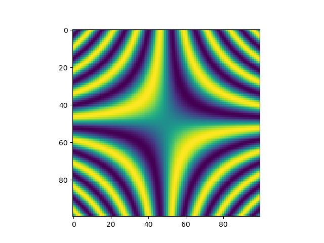
Figure 4.10 Application of the mesh grid in a two-dimensional representation of the function \(\sin(xy)\).

Making use of broadcasting, one can reduce the memory requirement by creating an open mesh grid instead:

>>> np.ogrid[0:2:3j, 0:1:5j]
[array([[0.],
       [1.],
       [2.]]), array([[0.  , 0.25, 0.5 , 0.75, 1.  ]])]

The function ogrid returns two two-dimensional arrays where one dimension is of length 1. Figure 4.11 shows an application to Bessel functions obtained by means of the following code:

>>> from scipy.special import jv
>>> nu, x = np.ogrid[0:10:41j, 0:20:100j]
>>> plt.imshow(jv(nu, x), origin='lower')
<matplotlib.image.AxesImage object at 0x7fde903736d8>
>>> plt.xlabel('$x$')
Text(0.5,0,'$x$')
>>> plt.ylabel(r'$\nu$')
Text(0,0.5,'$\\nu$')
>>> plt.show()

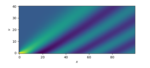
Figure 4.11 Two-dimensional plot of the family of Bessel functions \(J_\nu(x)\) of order \(\nu\) created by means of an open mesh grid created by ogrid.

Instead of using the ogrid function, one can also construct the argument arrays by hand. In this case, one has to take care of adding an additional axis in one of the two arrays as in the following example which results in Figure 4.12:

>>> x = np.linspace(-40, 40, 500)
>>> y = x[:, np.newaxis]
>>> z = np.sin(np.hypot(x-10, y))+np.sin(np.hypot(x+10, y))
>>> plt.imshow(z)
<matplotlib.image.AxesImage object at 0x7fde92509278>
>>> plt.show()

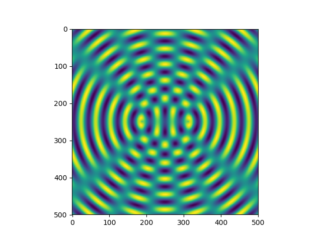
Figure 4.12 Interference pattern created with argument arrays obtained by means of linspace and by adding an additional axis in one of the two arrays. The function hypot determines the distance of the point given by the two argument coordinates from the origin.

So far, we have considered universal functions mostly as a convenient way to apply a function to an entire array. However, they can also make a significant contribution to speed up code. The following script compares the runtime between a for loop evaluating the sine function taken from the math module and a direct evaluation of the sine taken from NumPy for different array sizes:

import math
import matplotlib.pyplot as plt
import numpy as np
import time

def sin_math(nmax):
    xvals = np.linspace(0, 2*np.pi, nmax)
    start = time.time()
    for x in xvals:
        y = math.sin(x)
    return time.time()-start

def sin_numpy(nmax):
    xvals = np.linspace(0, 2*np.pi, nmax)
    start = time.time()
    yvals = np.sin(xvals)
    return time.time()-start

maxpower = 26
nvals = 2**np.arange(0, maxpower+1)
tvals = np.empty_like(nvals)
for nr, nmax in enumerate(nvals):
    tvals[nr] = sin_math(nmax)/sin_numpy(nmax)
plt.rc('text', usetex=True)
plt.xscale('log')
plt.yscale('log')
plt.xlabel('$n_\mathrm{max}$', fontsize=20)
plt.ylabel('$t_\mathrm{math}/t_\mathrm{numpy}$', fontsize=20)
plt.plot(nvals, tvals, 'o')
plt.show()

The results are presented in Figure 4.13 and depend on various factors including the hardware and details of the software environment. The data should therefore give a rough indication of the speedup and should not be taken too literally. The first point to note is that even for an array of size 1, NumPy is faster than the sine function taken from the math module. This seems to contradict our previous result on a scalar argument, but can be explained by the presence of the for loop in the sin_math function which results in an overhead even if the for loop is strictly speaking unnecessary. Then, for arrays of an intermediate size, a speed up of roughly a factor of 7 is observed. Interestingly, for array sizes beyond a few times \(10^4\), the speed up reaches values of around 100. This behavior can be explained by the use of the Anaconda distribution where NumPy is compiled to support Intel’s math kernel library (MKL). Even without this effect, a speed up between 5 and 10 may be significant enough to seriously consider the use of universal functions.

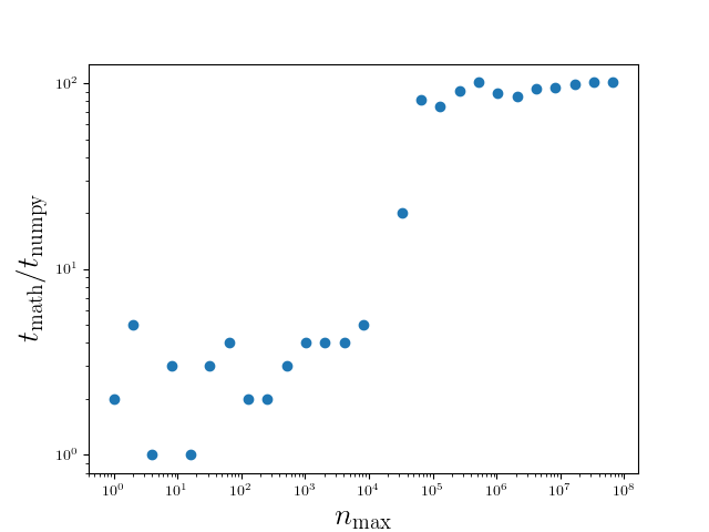
Figure 4.13 Runtime comparison between the sine function taken from the math module and from the NumPy package as a function of the array size. Larger values of the time ratio imply a larger speed up gained by means of NumPy. The data have been obtained by a version of NumPy with MKL support.

4.2.7. Linear algebra

Scientific problems which can be formulated in terms of vectors or matrices often require tools of linear algebra. Therefore, we will discuss a few of the more important functions NumPy has to offer in that domain. For more details we recommend to take a look at the documentation of the numpy.linalg module.

As we have discussed earlier, the usual multiplication operator does element-wise multiplication and uses broadcasting where applicable. The multiplication of arrays can either be done by means of the dot method or the @ operator:

>>> v1 = np.array([1, 2])
>>> v2 = np.array([3, 4])
>>> np.dot(v1, v2)
11
>>> m = np.array([[5, 6], [7, 8]])
>>> np.dot(m, v1)
array([17, 23])
>>> m @ v1
array([17, 23])

For the following, we will need to load the numpy.linalg module first:

>>> import numpy.linalg as LA

Here we have once more introduced a commonly used abbreviation. A vector can easily be normalized by means of the norm function:

>>> v = np.array([1, -2, 3])
>>> n = LA.norm(v)
>>> n**2
14.0
>>> v_normalized = v/n
>>> LA.norm(v_normalized)
1.0

Applying the norm function to a multi-dimensional array will return the Frobenius or Hilbert-Schmid norm, i.e. the square root of the sum over the squares of all matrix elements.

Some of the operations provided by the numpy.linalg module can be applied to a whole set of arrays. An example is the determinant which mathematically is defined only for two-dimensional arrays. For a three-dimensional array, determinants are calculated for each value of the index of axis 0:

>>> m = np.arange(12).reshape(3, 2, 2)
>>> m
array([[[ 0,  1],
        [ 2,  3]],

       [[ 4,  5],
        [ 6,  7]],

       [[ 8,  9],
        [10, 11]]])
>>> LA.det(m)
array([-2., -2., -2.])

It is also possible to determine the inverse for several matrices at the same time. Trying to invert a non-invertible matrix will result in a numpy.linalg.linalg.LinAlgError exception.

An inhomogeneous system of linear equations ax=b with a matrix a and a vector b can in principle be solved by inverting the matrix:

>>> a = np.array([[2, -1], [-3, 2]])
>>> b = np.array([1, 2])
>>> x = np.dot(LA.inv(a), b)
>>> x
array([4., 7.])
>>> np.dot(a, x)
array([1., 2.])

In the last command, we verified that the solution obtained one line above is indeed correct. Solving inhomogeneous systems of linear equations by inversion is however not very efficient and NumPy offers an alternative way based on an LU decomposition:

>>> LA.solve(a, b)
array([4., 7.])

As we have seen above for the determinant, the function solve also allows to solve several inhomogeneous systems of linear equations in one function call.

A frequent task in scientific applications is to solve an eigenvalue problem. The function eig determines the right eigenvectors and the associated eigenvalues for arbitrary square matrices:

>>> a = np.array([[1, 3], [4, -1]])
>>> evals, evecs = LA.eig(a)
>>> evals
array([ 3.60555128, -3.60555128])
>>> evecs
array([[ 0.75499722, -0.54580557],
       [ 0.65572799,  0.83791185]])
>>> for n in range(evecs.shape[0]):
...     print(np.dot(a, evecs[:, n]), evals[n]*evecs[:, n])
...
[2.72218119 2.36426089] [2.72218119 2.36426089]
[ 1.96792999 -3.02113415] [ 1.96792999 -3.02113415]

In the for loop, we compare the product of matrix and eigenvector with the corresponding product of eigenvalue and eigenvector and can verify that the results are indeed correct. In the matrix of eigenvectors, the eigenvectors are given by the columns.

Occasionally, it is sufficient to know the eigenvalues. In order to reduce the compute time, one can then replace eig by eigvals:

>>> LA.eigvals(a)
array([ 3.60555128, -3.60555128])

In many applications, the matrices appearing in eigenvalue problems are either symmetric of Hermitian. For these cases, NumPy provides the functions eigh and eigvalsh. One advantage is that it suffices to store only half of the matrix elements. More importantly, these specialized functions are much faster:

>>> import timeit
>>> a = np.random.random(250000).reshape(500, 500)
>>> a = a+a.T
>>> timeit.repeat('LA.eig(a)', number=100, globals=globals())
[13.307299479999529, 13.404196323999713, 13.798628489999828]
>>> timeit.repeat('LA.eigh(a)', number=100, globals=globals())
[1.8066274120001253, 1.7375857540000652, 1.739574907000133]

In the third line, we have made sure that the initial random matrix is turned into a symmetric matrix by adding its transpose. In this example, we observe a speedup of about a factor of 7.

4.3. SciPy

The functions offered through the SciPy package cover many tasks typically encountered in the numerical treatment of scientific problems. Here, we can only give an impression of the potential of SciPy by discussing a few examples. It is highly recommended to take a look at the SciPy API Reference.

As a first example, we consider the linear regression of noisy data. In a first step, we create data on a line with normally distributed noise added on top:

>>> x = np.linspace(0, 10, 101)
>>> y = 2*x + 1 + np.random.normal(0, 1, 101)

Now, we can use the linregress function from the statistical functions module of SciPy to do a least-squares regression of the noisy data:

>>> from scipy.stats import linregress
>>> slope, intercept, rvalue, pvalue, stderr = linregress(x, y)
>>> plt.plot(x, y, 'o')
>>> plt.plot(x, slope*x + intercept)
>>> plt.show()
>>> print(rvalue, stderr)
0.9853966954685487 0.0350427823008272

Here rvalue refers to the correlation coefficient and stderr is the standard error of the estimated gradient. The graph containing the noisy data and the linear fit is shown in Figure 4.14.

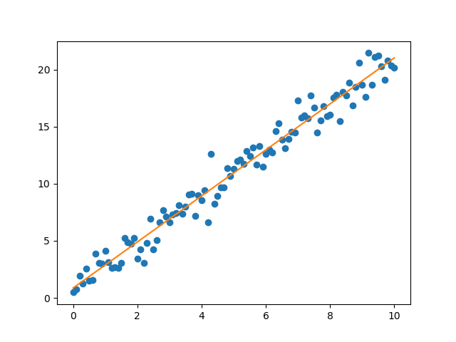
Figure 4.14 Noisy data (blue points) and result of the linear regression (orange line) obtained by means of scipy.stats.linregress.

Fitting of data cannot always be reduced to linear regression. Then we can resort to the curve_fit function from the optimization module of SciPy:

>>> from scipy.optimize import curve_fit
>>> def fitfunc(x, a, b):
...     return a*np.sin(x+b)
...
>>> x = np.linspace(0, 10, 101)
>>> y = 2*np.sin(x+0.5) + np.random.normal(0, 1, 101)
>>> plt.plot(x, y, 'o')
>>> popt, pcov = curve_fit(fitfunc, x, y)
>>> popt
array([2.08496412, 0.43937489])
>>> plt.plot(x, popt[0]*np.sin(x+popt[1]))
>>> plt.show()

In order to fit to a general function, one needs to provide curve_fit with a function, called fitfunc here, which depends on the variable as well as a set of parameters. In our example, we have chosen two parameters a and b but we are in principle not limited to this number. However, as the number of parameters increases, the fit tends to become less reliable. The fit values for the parameters are returned in the array popt together with the covariance matrix for the parameters pcov. The outcome of the fit is shown in Figure 4.15.

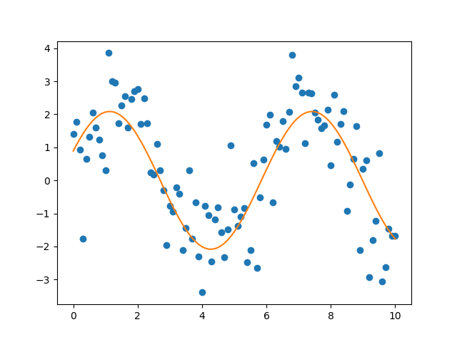
Figure 4.15 Fit of a noisy sine function by means of scipy.optimize.curve_fit.

Occasionally, a root search is required. As an example, we consider the determination of the ground state energy in a finite potential well. The eigenvalue condition for a symmetric eigenstate reads

\[\sqrt{\epsilon}\cos(\alpha\sqrt{1-\epsilon})-\sqrt{1-\epsilon}\sin(\alpha\sqrt{1-\epsilon})=0\,,\]

where \(\epsilon\) is the energy in units of the well depth and \(\alpha\) is a measure of the potential strength combining the well depth and its width. One way of solving this nonlinear equation for \(\epsilon\) is by means of the brentq function, which needs at least the function of which the root should be determined as well as the bounds of an interval in which the function changes its sign. If the potential well is sufficiently shallow, i.e. if :math.``alpha`` is sufficiently small, the left-hand side contains only one root as can be seen from the blue line in Figure 4.16. In our example, the function requires an additional argument \(\alpha\) which also needs to be given to brentq. Finally, in order to know how many iterations are need, we set full_output to True.

>>> from scipy.optimize import brentq
>>> def f(energy, alpha):
...     sqrt_1me = np.sqrt(1-energy)
...     return (np.sqrt(energy)*np.cos(alpha*sqrt_1me)
...             -sqrt_1me*np.sin(alpha*sqrt_1me))
...
>>> alpha = 1
>>> x0, r = brentq(f, a=0, b=1, args=alpha, full_output=True)
>>> x0
>>> 0.45375316586032827
>>> r
       converged: True
           flag: 'converged'
 function_calls: 7
     iterations: 6
           root: 0.45375316586032827)
>>> x = np.linspace(0, 1, 400)
>>> plt.plot(x, f(x, alpha))
>>> plt.plot(x0, 0, 'o')
>>> plt.show()

As the output indicates, the root is found within 6 iterations. The resulting root is depicted in Figure 4.16 as an orange dot.

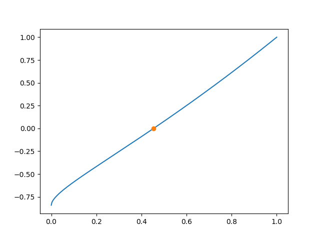
Figure 4.16 Determination of the ground state energy in a finite potential well of depth \(\alpha=1\) by means of scipy.optimize.brentq.

Finally, we consider a more complex example which involves optimization and the solution of a coupled set of differential equations. The physical problem to be studied numerically is the fall of a chain where the equations of motion are derived in W. Tomaszweski, P. Pieranski, and J.-C. Geminard, Am. J. Phys. 74, 776 (2006) [9] and account for damping inside the chain. For the initial configuration of the chain, we take a chain hanging in equilibrium where the two ends are at equal height and at a given horizontal distance. In the continuum limit, the chain follows a catenary, but in the discrete case treated here, we obtain the equilibrium configuration by optimizing the potential energy. This is done in the method equilibrium of our Chain class. The method essentially consists of a call to the minimize function taken from the optimize module of SciPy. It optimizes the potential energy defined in the f_energy method. In addition, we have to account for two constraints corresponding to the horizontal and vertical direction and implemented through the methods x_constraint and y_constraint. An example of the result of this optimization procedure is depicted in Figure 4.17 for a chain made of 9 links.

import numpy as np
import numpy.linalg as LA
import matplotlib.pyplot as plt
from scipy.optimize import minimize
from scipy.integrate import solve_ivp

class Chain:
    def __init__(self, nlinks, length, damping):
        if nlinks < length:
            raise ValueError('length requirement cannot be fulfilled with '
                             'the given number of links')
        self.nlinks = nlinks
        self.length = length
        self.m = self.matrix_m()
        self.a = self.vector_a()
        self.damping = (-2*np.identity(self.nlinks, dtype=np.float64)
                          +np.eye(self.nlinks, k=1)
                          +np.eye(self.nlinks, k=-1))
        self.damping[0, 0] = -1
        self.damping[self.nlinks-1, self.nlinks-1] = -1
        self.damping = damping*self.damping

    def x_constraint(self, phi):
        return np.sum(np.cos(phi))-self.length

    def y_constraint(self, phi):
        return np.sum(np.sin(phi))

    def f_energy(self, phi):
        return np.sum(np.arange(self.nlinks, 0, -1)*np.sin(phi))

    def equilibrium(self):
        result = minimize(self.f_energy, np.linspace(-0.1, 0.1, self.nlinks),
                          method='SLSQP',
                          constraints=[{'type': 'eq', 'fun': self.x_constraint},
                                       {'type': 'eq', 'fun': self.y_constraint}])
        return result.x

    def plot_equilibrium(self):
        phis = chain.equilibrium()
        x = np.zeros(chain.nlinks+1)
        x[1:] = np.cumsum(np.cos(phis))
        y = np.zeros(chain.nlinks+1)
        y[1:] = np.cumsum(np.sin(phis))
        plt.plot(x, y)
        plt.plot(x, y, 'o')
        plt.axes().set_aspect('equal')
        plt.show()

    def matrix_m(self):
        m = np.fromfunction(lambda i, j: self.nlinks-np.maximum(i, j)-0.5,
                            (self.nlinks, self.nlinks), dtype=np.float64)
        m = m-np.identity(self.nlinks)/6
        return m

    def vector_a(self):
        a = np.arange(self.nlinks, 0, -1)-0.5
        return a

    def diff(self, t, y):
        momenta = y[:self.nlinks]
        angles = y[self.nlinks:]
        d_angles = momenta
        ci = np.cos(angles)
        cij = np.cos(angles[:,np.newaxis]-angles)
        sij = np.sin(angles[:,np.newaxis]-angles)
        mcinv = LA.inv(self.m*cij)
        d_momenta = -np.dot(self.m*sij, momenta*momenta)
        d_momenta = d_momenta+np.dot(self.damping, momenta)
        d_momenta = d_momenta-self.a*ci
        d_momenta = np.dot(mcinv, d_momenta)
        d = np.empty_like(y)
        d[:self.nlinks] = d_momenta
        d[self.nlinks:] = d_angles
        return d

    def solve_eq_of_motion(self, time_i, time_f, nt):
        y0 = np.zeros(2*self.nlinks, dtype=np.float64)
        y0[self.nlinks:] = self.equilibrium()
        self.solution = solve_ivp(self.diff, (time_i, time_f), y0, method='Radau',
                                  t_eval=np.linspace(time_i, time_f, nt))

    def plot_dynamics(self):
        for i in range(self.solution.y.shape[1]):
            phis = self.solution.y[:, i][self.nlinks:]
            x = np.zeros(self.nlinks+1)
            x[1:] = np.cumsum(np.cos(phis))
            y = np.zeros(self.nlinks+1)
            y[1:] = np.cumsum(np.sin(phis))
            plt.plot(x, y, 'b')
        plt.axes().set_aspect('equal')
        plt.show()

chain = Chain(200, 150, 0.003)
chain.solve_eq_of_motion(0, 40, 50)
chain.plot_dynamics()

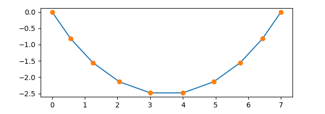
Figure 4.17 Chain consisting of 9 links hanging in its equilibrium position with a horizontal distance of the ends equivalent to the length of 7 links.

In a second step, the equation of motion for the chain links is solved in the solve_eq_of_motion method by means of solve_ivp taken from the integrate module of SciPy. We need to express the second order equations of motion in terms of first-order differential equations which can always be achieved by doubling the number of degrees of freedom by means of auxiliary variables. The main ingredient then is the function called diff in our example which for a given set of variables returns the time derivatives for these variables. Furthermore, solve_ivp needs to know the time interval on which the solution is to be determined together with the time values for which a solution is requested as well as the initial configuration. Finally, out of the various solvers, we choose Radau which implements an implicit Runge-Kutta method of Radau IIA family of order 5. Figure 4.18 displays a stroboscopic plot of the chain during is first half period swinging from the right to the left.

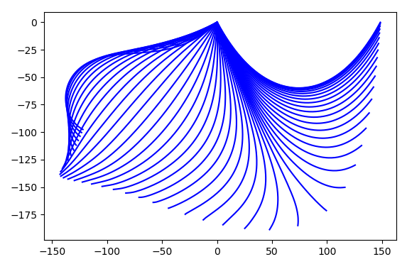
Figure 4.18 Stroboscopic image of a falling chain consisting of 200 elements starting out from its equilibrium state in the upper right during its first half period swinging to the left.

[1]

For details see the NumPy Reference.

[2]

For details see the SciPy API Reference.

[3]

See the matplotlib gallery to obtain an idea of the possibilities offered by matplotlib.

[4]

For details see the homepage of the Jupyter project.

[5]

For details see the pandas homepage.

[6]

For details see the sympy homepage.

[7]

For details see the scikit-image homepage.

[8]

For details see the scikit-learn homepage.

[9]

doi:10.1119/1.2204074.