7. Aspects of parallel computing

Today even consumer computers are equipped with multi-core processors which allow to run programs truly in parallel. In numerical calculations, algorithms can often be parallelized so that the execution time can be reduced by running the code on several compute cores. A program could thus profit from the use of several cores within a single processor or from a potentially large number of cores in a computer cluster accommodating a large number of processors.

Parallel execution of a program can result in problems if the individual computations are not well synchronized among each other. The final result might then depend on how fast each of the computations is carried out. Such racing conditions may lead to problems which are sometimes difficult to debug. CPython, the most popular implementation of Python, therefore implements the so-called Global Interpreter Lock (GIL) which prevents actual parallel execution within a single Python process. This aspect will be discussed further in the following section.

Despite the GIL, parallel processing is possible in Python if several processes is started. In Section 7.2, we will demonstrate how this can be done by considering the calculation of the Mandelbrot set as an example. This problem is particularly simple because it allows to decompose the full problem into smaller problems without requiring any exchange of data between them. This kind of problems is referred to as embarrassingly parallel. Here, we will restrict ourselves to this type of problems. The communication between processes running in parallel raises a number of difficulties which are beyond the scope of the present lecture notes. Readers interested more deeply in this topic might want to read more on the message passing interface (MPI) and take a look at the mpi4py package.

In the last section of this chapter, we will address the possibilities offered by Numba, a so-called Just in Time Compiler (JIT Compiler). The use of Numba can lead to significant improvements of the run time of a program. Furthermore, Numba can support the parallel handling of Python code.

7.1. Threads, processes and the GIL

Modern operating systems can seemingly run several tasks in parallel even on a simple compute core. In practice, this is achieved by in turn allotting compute time to different tasks so that a single task usually cannot block other tasks from execution over a longer period of time.

It is important to distinguish two different kinds of tasks: processes and threads. Processes have at their disposal a reserved range of memory and their own access to other system resources. As a consequence, starting a new process comes with a certain overhead in time. A single process will start first one and subsequently possibly further threads in order to handle different tasks. Threads differ from processes by working on the same range of memory and by accessing the same system resources. Starting a thread is thus less demanding than starting a process.

Since threads share a common range of memory, they can access the same data and easily exchange data among each other. Communication between different threads thus leads to very little overhead. However, the access to common data is not without risks. If one does not take care that reading and writing data by different threads is done in the intended order, it may happen that a thread does not obtain the data it needs. As the occurrence of such mistakes depends on details of which thread executes which tasks at a given time, such problems are not easily reproducible and sometimes quite difficult to identify. There exist techniques to cope with the difficulties involved in the communication between different threads, making multithreading, i.e. the parallel treatment in several threads, possible. We will, however, not cover these techniques in the present lecture notes.

As already mentioned in the introduction, the most popular implementation of Python, CPython implemented in C, makes use of the GIL, the global interpreter lock. The GIL prevents a single Python process to execute more than one thread in parallel. While it is possible to make use of multithreading in Python [1], the GIL will ensure that individual threads will never run in parallel but in turn are allotted their slots of compute time. In this way, only an illusion of parallel processing is created.

If the time of execution of a Python script is limited by the compute time, multithreading will not result an in improvement. To the contrary, the overhead arising from the necessity to change between different threads will lead to a slow-down of the script. However, there exist scripts which are I/O-bound. An example could be a script processing data which need to be downloaded from the internet. While a thread is waiting for new data to arrive, another thread might use the time to process data already available. For I/O-bounded scripts, multithreading thus may be a good strategy even in Python.

However, numerical programs are usually not I/O-bound but limited by the compute time. Therefore, we will not consider multithreading any further but rather concentrate on multiprocessing, i.e. parallel treatment by means of several Python processes. It is worth mentioning though that multithreading may play a role even in numerical applications written in Python when numerical libraries are used. Such libraries are often based on C code which is not subject to the restrictions imposed by the GIL. Linear algebra routines provided by an appropriately compiled version of NumPy may serve as an example. This includes the NumPy library available through the Anaconda distribution which is compiled with the Intel® Math Kernel Library (MKL). Figure 7.1 demonstrates an example where four cores are used when determining the eigenvectors and eigenvalues of a large matrix. Another option to circumvent the GIL is offered by Cython [2] which allows to generate C extensions from Python code. Those parts of the code not accessing Python objects can then be executed in a nogil context outside the control of the GIL.

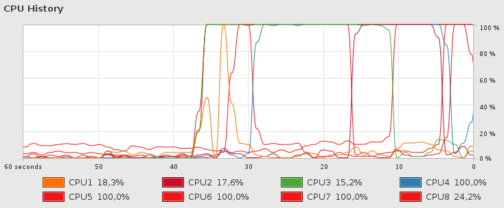
Figure 7.1 In this example, the graph of the system load shows that during the solution of the eigenvalue problem for a large matrix by means of NumPy compiled with the Intel® MKL four cores are used at the same time.

7.2. Parallel computing in Python

We will illustrate the use of parallel processes in Python by considering a specific example, namely the calculation of the Mandelbrot set. Mathematically, the Mandelbrot set is defined as the set of complex numbers \(c\) for which the series generated by the iteration

\[z_{n+1} = z_n^2+c\]

with the initial value \(z_0=0\) remains bounded. It is known that the series is not bound once \(\vert z\vert>2\) has been reached so that it suffices to perform the iteration until this threshold has been reached. The iterations for different values of \(c\) can be performed completely independently of each other so that it is straightforward to distribute different values of \(c\) to different processes. The problem is thus embarrassingly parallel. Once all individual calculations are finished, it suffices to collect all data and to represent them graphically.

We start out with the following initial version of a Python script to determine the Mandelbrot set.

import time
import numpy as np
import matplotlib.pyplot as plt

def mandelbrot_iteration(cx, cy, nitermax):
    x = 0
    y = 0
    for n in range(nitermax):
        x2 = x*x
        y2 = y*y
        if x2+y2 > 4:
            return n
        x, y = x2-y2+cx, 2*x*y+cy
    return nitermax

def mandelbrot(xmin, xmax, ymin, ymax, npts, nitermax):
    data = np.empty(shape=(npts, npts), dtype=np.int)
    dx = (xmax-xmin)/(npts-1)
    dy = (ymax-ymin)/(npts-1)
    for nx in range(npts):
        x = xmin+nx*dx
        for ny in range(npts):
            y = ymin+ny*dy
            data[ny, nx] = mandelbrot_iteration(x, y, nitermax)
    return data

def plot(data):
    plt.imshow(data, extent=(xmin, xmax, ymin, ymax),
               cmap='jet', origin='bottom', interpolation='none')
    plt.show()

nitermax = 2000
npts = 1024
xmin = -2
xmax = 1
ymin = -1.5
ymax = 1.5
start = time.time()
data = mandelbrot(xmin, xmax, ymin, ymax, npts, nitermax)
ende = time.time()
print(ende-start)
plot(data)

Here, the iteration prescription is carried out in the function mandelbrot_iteration up to maximum number of iterations given by nitermax. We handle real and imaginary parts separately instead of performing the iteration with complex numbers. It turns out that our choice is slightly faster, but more importantly, this approach can also be employed for the NumPy version which we are going to discuss next.

The purpose of the function mandelbrot is to walk through a grid of complex values \(c\) and to collect the results in the array data. For simple testing purposes, it is useful to graphically represent the results by means of the function plot. We also have added code to determine the time spent in the functions mandelbrot and mandelbrot_iteration. On an i7-6700HQ CPU, we measured and execution time of 81.1 seconds.

Before parallelizing code, it often makes sense to consider other possible improvements. In our case, it is natural to take a look at a version making use of NumPy. Here, we list only the code replacing the functions mandelbrot and mandelbrot_iteration in our first version.

def mandelbrot(xmin, xmax, ymin, ymax, npts, nitermax):
    cy, cx = np.mgrid[ymin:ymax:npts*1j, xmin:xmax:npts*1j]
    x = np.zeros_like(cx)
    y = np.zeros_like(cx)
    data = np.zeros(cx.shape, dtype=np.int)
    for n in range(nitermax):
        x2 = x*x
        y2 = y*y
        notdone = x2+y2 < 4
        data[notdone] = n
        x[notdone], y[notdone] = (x2[notdone]-y2[notdone]+cx[notdone],
                                  2*x[notdone]*y[notdone]+cy[notdone])
    return data

For an appealing graphical representation of the Mandelbrot set, we need to keep track of the number of iterations required to reach the threshold for the absolute value of \(z\). We achieve this by fancy indexing with the array notdone. An entry of True means that the threshold has not been reached yet. An example of the graphical output generated by the NumPy version of the program is shown in Figure 7.2.

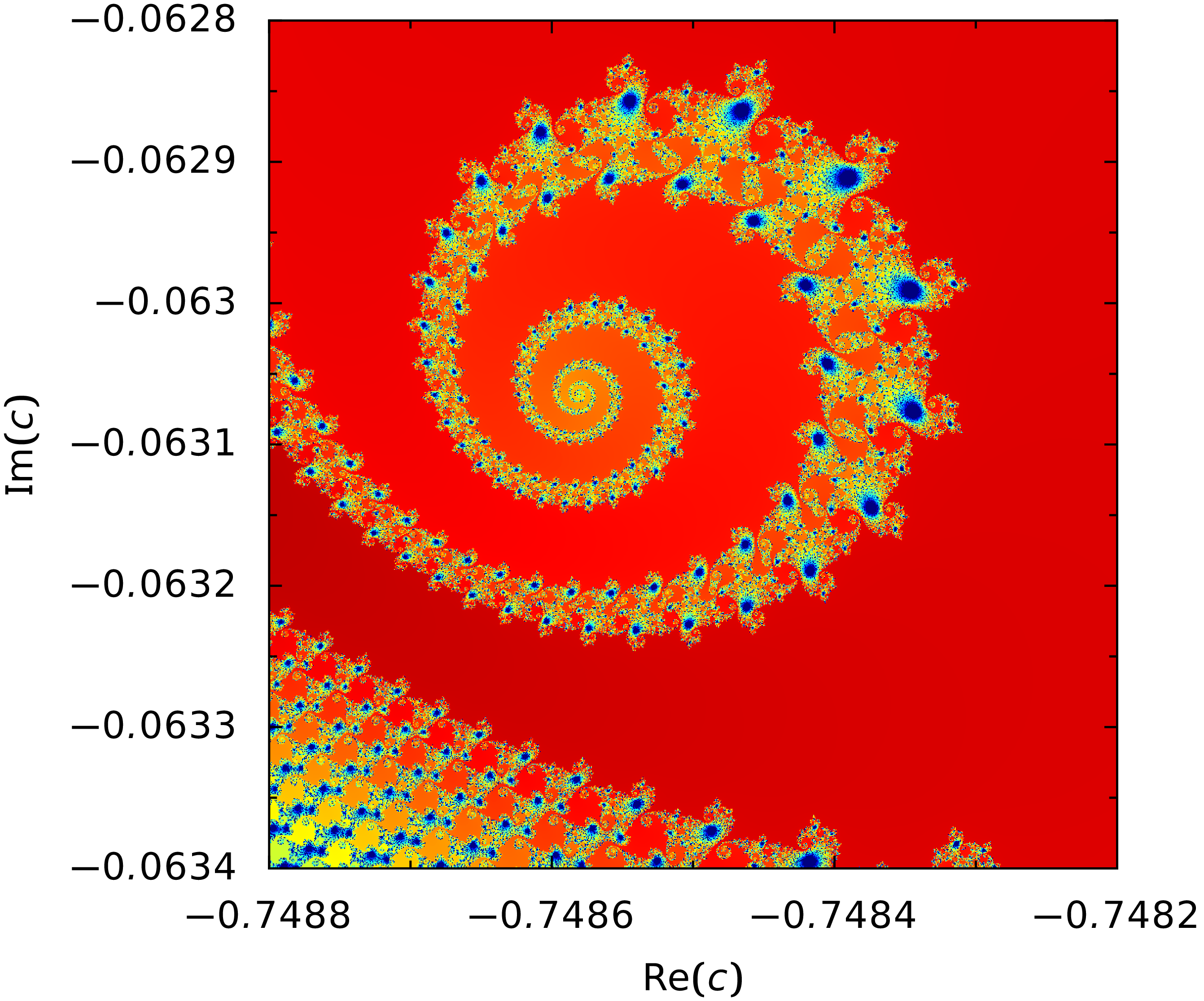
Figure 7.2 Detail of the Mandelbrot set where the color represents the number of iterations needed until the threshold of 2 for the absolute value of \(z\) is reached.

For the NumPy version, we have measured an execution time of 22.8s, i.e. almost a factor of 3.6 faster than our initial version.

Now, we will further accelerate the computation by splitting the task into several parts which will be attributed to a number of processes for processing. For this purpose, we will make use of the module concurrent.futures available from the Python standard library. The name concurrent indicates that several tasks are carried out at the same time while futures refers to objects which will provide the desired results at a later time.

For a parallel computation of the Mandelbrot set, we decompose the area in the complex plane covering the relevant values of \(c\) into tiles, which will be treated separately by the different processes. Figure 7.3 displays a distribution of 64 tiles on four processes indicated by different colors. Since the processing time for the tiles differs, there is one process which has treated only 15 tiles while another process has treated 17.

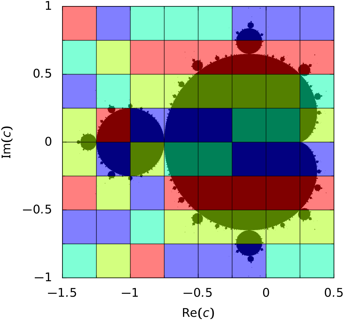
Figure 7.3 The four different colors indicate which one out of four processes has carried out the computation for the corresponding tile. Note that the number of tiles per process does not necessarily equal 16.

The following code demonstrates how the NumPy based version can be adapted to a parallel treatment. Again we concentrate on the Mandelbrot specific parts.

from concurrent import futures
from itertools import product
from functools import partial

import numpy as np

def mandelbrot_tile(nitermax, nx, ny, cx, cy):
    x = np.zeros_like(cx)
    y = np.zeros_like(cx)
    data = np.zeros(cx.shape, dtype=np.int)
    for n in range(nitermax):
        x2 = x*x
        y2 = y*y
        notdone = x2+y2 < 4
        data[notdone] = n
        x[notdone], y[notdone] = (x2[notdone]-y2[notdone]+cx[notdone],
                                  2*x[notdone]*y[notdone]+cy[notdone])
    return (nx, ny, data)

def mandelbrot(xmin, xmax, ymin, ymax, npts, nitermax, ndiv, max_workers=4):
    cy, cx = np.mgrid[ymin:ymax:npts*1j, xmin:xmax:npts*1j]
    nlen = npts//ndiv
    paramlist = [(nx, ny,
                  cx[nx*nlen:(nx+1)*nlen, ny*nlen:(ny+1)*nlen],
                  cy[nx*nlen:(nx+1)*nlen, ny*nlen:(ny+1)*nlen])
                 for nx, ny in product(range(ndiv), repeat=2)]
    with futures.ProcessPoolExecutor(max_workers=max_workers) as executors:
        wait_for = [executors.submit(partial(mandelbrot_tile, nitermax),
                                             nx, ny, cx, cy)
                    for (nx, ny, cx, cy) in paramlist]
        results = [f.result() for f in futures.as_completed(wait_for)]
    data = np.zeros(cx.shape, dtype=np.int)
    for nx, ny, result in results:
        data[nx*nlen:(nx+1)*nlen, ny*nlen:(ny+1)*nlen] = result
    return data

The main changes have occurred in the function mandelbrot. In addition to the arguments present already in earlier versions, two arguments have been added: ndiv and max_workers. ndiv defines the number of divisions in each dimension of the complex plane. In the example of Figure 7.3, ndiv was set to 8, resulting in 64 tiles. The argument max_workers defines the maximal number of processes which will run under the control of our script. The choice for this argument will depend on the number of cores available to the script.

In lines 23-26, we define a list of parameters characterizing the individual tiles. Each entry contains the coordinates (nx, ny) of the tile which will later be needed to collect all data. In addition, the section of the real and imaginary parts of \(c\) corresponding to the tile become part of the parameter list. The double loop required in the list comprehension is simplified by making use of the product method available from the itertools module of the Python standard library imported in line 2.

The main part responsible for the distribution of tasks to the different workers can be found in lines 27-31. This code runs under the control of a context manager which allocates a pool of max_workers executors. The method ProcessPoolExecutor is available from the concurrent.futures module.

In lines 28-30 a list of tasks is submitted to the executors. Each submission consists of a function, in our case mandelbrot_tile, and the corresponding parameters. The function mandelbrot_tile possesses one argument nitermax which is the same for all tasks and the parameters listed in paramlist which differ from task to task. Therefore, we construct a partial function object which fixes nitermax and requires only nx, ny, cx, and cy as arguments. The partial method is imported from the functools module in line 3.

In line 31, the results are collected in a list comprehension. Once all tasks have been completed, the list results contains entries consisting of the coordinates (nx, ny) of the tile and the corresponding data as defined in line 18. In lines 33-34, the data are brought into order to fill the final array data which subsequently can be used to produce graphical output.

It is interesting to study how the total time to determine the Mandelbrot set depends on the number of tiles. The corresponding data are shown in Figure 7.4 for four parallel processes. In the case of four tiles, we see that the different tiles require different times so that we have to wait for the slowest process. For four tiles, where the memory requirement per process is relatively large, we also can see a significant time needed to start a process. Increasing the number of tiles leads to a reduction of the execution time. However, even for 16 tiles, one has to wait for the last process. The optimum for four processes is reached for 64 tiles. Increasing the number of tiles further will lead to an increasing overhead when switching from one task to the next.

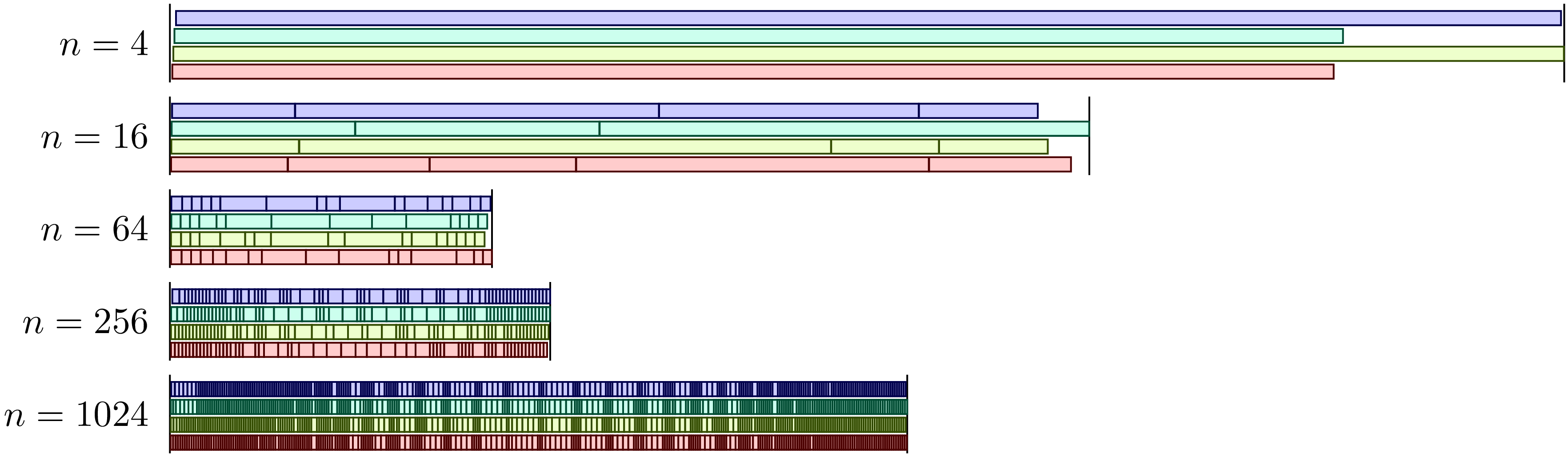
Figure 7.4 Distribution of tasks to determine the Mandelbrot set over four processes as a function of the number of tiles.

Figure 7.5 depicts the acceleration for four processes as a function of the number of divisions per axis. The points connected by the dotted line are obtained by dividing the time required by a single process without subdividing the task through the time required by four processes with the subdivision indicated in the figure. In agreement with Figure 7.4 we find the largest acceleration for 8 divisions per axis, i.e. 64 tiles. Interestingly, the acceleration can reach values slightly exceeding a factor six. This effect may result from a more effective use of caches for smaller problems as compared to the full problem with \(n=1\). The effect of caches can be excluded by taking ratio of the execution times for one and four processes for the same number of tiles. As Figure 7.5 demonstrates, a factor of nearly four is reached beyond \(n=8\).

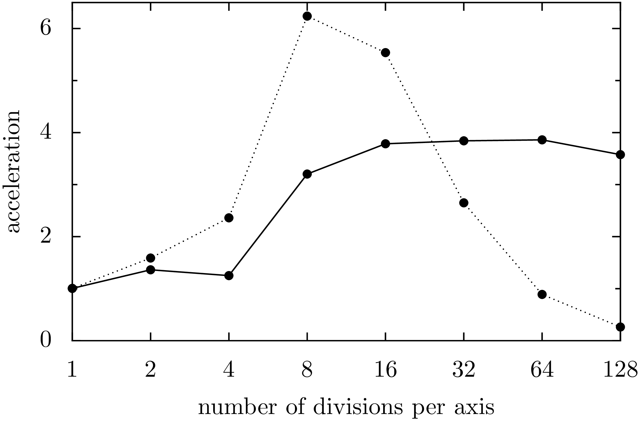
Figure 7.5 Acceleration by parallelization in the computation of the Mandelbrot set with four processes as a function of the number of divisions per axis. The points connected by the dotted line represent the acceleration of the parallelized version with respect to the unparallelized version without subdivision. The points connected by the full line represent the acceleration of the parallelized version with respect to the unparallelized version for the same number of divisions.

7.3. Numba

In the previous section we have seen how a program can be accelerated by means of NumPy and parallelization. For our example of the Mandelbrot set, this could be achieved in a rather straightforward manner because the use of arrays came quite naturally and parallelization did not require any communication between the different tasks. Besides the use of NumPy and parallelization of the code, there exist other options to accelerate Python scripts, some of them being very actively developed at present. Therefore, we do not attempt a complete description but rather highlight some ways to accelerate a Python script.

We will specifically discuss Numba [3] because it is designed to work with NumPy and also supports parallelization. Numba makes use of just in time (JIT) compilation. While Python scripts usually are interpreted, Numba will produce executable code for a function when it is called first. The compilation step implies a certain investment of time but the function can be executed faster during subsequent calls. Python allows to call functions with different signatures, i.e. the data types of the arguments are not fixed. Compiled code, on the other hand, depends on the signature. Therefore, additional compilation steps may become necessary.

We will demonstrate just in time compilation and the effect of different signatures by approximately determining the Riemann zeta function

\[\zeta(s) = \sum_{n=1}^\infty\frac{1}{n^s}\,.\]

The following implementation of the code is not particularly well suited to efficiently determine the zeta function but this is not relevant for our discussion. Without using Numba, a direct implementation of the sum looks as follows:

def zeta(x, nmax):
    zetasum = 0
    for n in range(1, nmax+1):
        zetasum = zetasum+1/(n**x)
    return zetasum

print(zeta(2, 100000000))

We can now simply make use of Numba by importing it in line 1 and adding a decorator numba.jit to the function zeta:

import numba

@numba.jit
def zeta(x, nmax):
    zetasum = 0
    for n in range(1, nmax+1):
        zetasum = zetasum+1/(n**x)
    return zetasum

print(zeta(2, 100000000))

Running the two pieces of code, we find an execution time for the first version of 34.1 seconds while the second version takes only 0.85 seconds. After running the code, we can print out the signatures for which the function zeta was compiled by Numba:

print(zeta.signatures)

Because we called the function with two integers as arguments, we obtain not unexpectedly:

[(int64, int64)]

Like in NumPy and in contrast to Python, integers cannot become arbitrarily large. In our example, they have a length of eight bytes. Accordingly, one has to beware of overflows. For example, if we set x to 3, we will encounter a division by zero.

To demonstrate that Numba compiles the function for each signature anew, we call zeta with an integer, a float, and a complex number:

import time
import numba

@numba.jit
def zeta(x, nmax):
    zetasum = 0
    for n in range(1, nmax+1):
        zetasum = zetasum+1/(n**x)
    return zetasum

nmax = 100000000
for x in (2, 2.5, 2+1j):
    start = time.time()
    print(f'ζ({x}) = {zeta(x, nmax)}')
    print(f'execution time: {time.time()-start:5.2f}s\n')

print(zeta.signatures)

The resulting output demonstrates that the execution time depends on the type of variable x` and that Numba has indeed compiled the function for three different signatures:

ζ(2) = 1.644934057834575
execution time:  0.59s

ζ(2.5) = 1.341487257103954
execution time:  5.52s

ζ((2+1j)) = (1.1503556987382961-0.43753086346605924j)
execution time: 13.41s

[(int64, int64), (float64, int64), (complex128, int64)]

Numba also allows us to transform functions into universal functions or ufuncs which we have introduced in Section 4.2.6. Besides scalar arguments, universal functions are capable of handling array arguments. This is achieved already by using the decorator jit. By means of the decorator vectorize, the evaluation of the function with an array argument can even by performed in several threads in parallel.

In the following code example, we specify the signature for which the function zeta should be compiled as argument of the decorator vectorize. The argument x is a float64 and can also be a corresponding array while n is an int64. The result is again a float64 and is listed as first argument before the pair of parentheses enclosing the arguments’ data type. The argument target is given the value 'parallel' so that in the case of an array argument the use of several threads is possible. If a parallel processing is not desired, for example because for a small task starting a thread would cost too much time, one can set target='cpu' instead. If an appropriate graphics processor is available, one might consider setting target='cuda'.

import numpy as np
from numba import vectorize, float64, int64

@vectorize([float64(float64, int64)], target='parallel')
def zeta(x, nmax):
    zetasum = 0.
    for n in range(nmax):
        zetasum = zetasum+1./((n+1)**x)
    return zetasum

x = np.linspace(2, 10, 200, dtype=np.float64)
y = zeta(x, 10000000)

Figure 7.6 shows how the execution time for the Riemann zeta function can be reduced by using more than one thread. The number of threads can be set by means of an environment variable. The following command sets the number of threads to four:

$ export NUMBA_NUM_THREADS=4; python zeta.py

The timing in Figure 7.6 was done on an i7-6700HQ processor with four cores and hyperthreading which allows to run eight threads in parallel. Up to four threads, the execution time decrease almost inversely proportional to the number of threads. Increasing the number of threads beyond the number of cores will further accelerate the execution but by a much smaller amount. The reason is that threads need to wait for free resources more often.

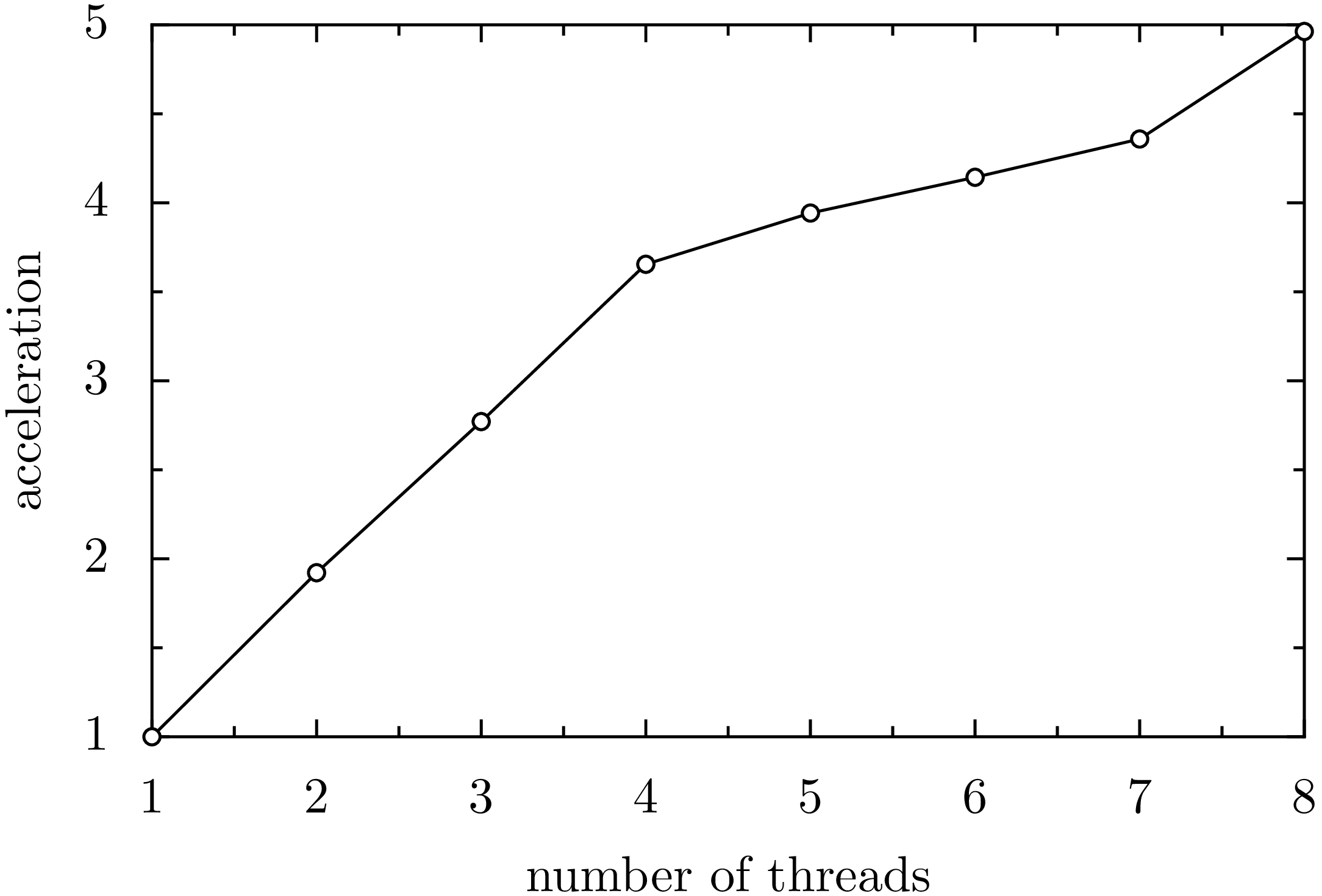
Figure 7.6 Acceleration of the computation of the Riemann zeta function as a function of the number of threads on a CPU with four cores and hyperthreading.

With Numba, universal functions can be further generalized by means of the decorator guvectorize so that not only scalars but also arrays can be employed in the inner loop. We will illustrate this by applying Numba to our Mandelbrot example.

from numba import jit, guvectorize, complex128, int64
import matplotlib.pyplot as plt
import numpy as np

@jit
def mandelbrot_iteration(c, maxiter):
    z = 0
    for n in range(maxiter):
        z = z**2+c
        if z.real*z.real+z.imag*z.imag > 4:
            return n
    return maxiter

@guvectorize([(complex128[:], int64[:], int64[:])], '(n), () -> (n)',
             target='parallel')
def mandelbrot(c, itermax, output):
    nitermax = itermax[0]
    for i in range(c.shape[0]):
        output[i] = mandelbrot_iteration(c[i], nitermax)

def mandelbrot_set(xmin, xmax, ymin, ymax, npts, nitermax):
    cy, cx = np.ogrid[ymin:ymax:npts*1j, xmin:xmax:npts*1j]
    c = cx+cy*1j
    return mandelbrot(c, nitermax)

def plot(data, xmin, xmax, ymin, ymax):
    plt.imshow(data, extent=(xmin, xmax, ymin, ymax),
               cmap='jet', origin='bottom', interpolation='none')
    plt.show()

nitermax = 2000
npts = 1024
xmin = -2
xmax = 1
ymin = -1.5
ymax = 1.5
data = mandelbrot_set(xmin, xmax, ymin, ymax, npts, nitermax)

Let us take a closer look at the function mandelbrot decorated by guvectorize which has a special set of arguments. The function mandelbrot possesses three arguments. However, only two of them are intended as input: c and itermax. The third argument output will contain the data returned by the function. This can be inferred from the second argument of the decorator, the so-called layout. The present layout indicates that the returned array output has the same shape as the input array c. Because c is a two-dimensional array, the argument c[i] of the function mandelbrot_iteration is again an array which can be handled by several threads. While maxiter in the function mandelbrot_iteration has to be a scalar, the array itermax is converted in line 17 into a scalar.

On the same processor on which we timed earlier version of the Mandelbrot program and which through hyperthreads supports up to eight threads, we find an execution time of 0.56 seconds. Compared to our fastest parallelized program, we thus observe an acceleration by more than a factor of six and compared to our very first version the present version is faster by a factor of almost 150.

[1]

When referring to Python, we always mean CPython. An example of an implementation of Python without a GIL is Jython written in Java.

[2]

Cython should not be confused with CPython, the C implementation of Python. More information on Cython can be found at https://cython.org/.

[3]

Up-to-date information on Numba can be found at https://numba.pydata.org/.